Estimate Model Parameters Using Time-Independent Data (Code)

Since R2023b

This example demonstrates the approach to estimate model parameters when the experimental data describes a time-independent X-Y relationship between two signals. The example showcases both unconstrained and constrained parameter estimation.

Wen-Bouc Model of Hysteric Spring

Open the hysteric spring model sdoWenBoucSpring.

model = "sdoWenBoucSpring";
open_system(model)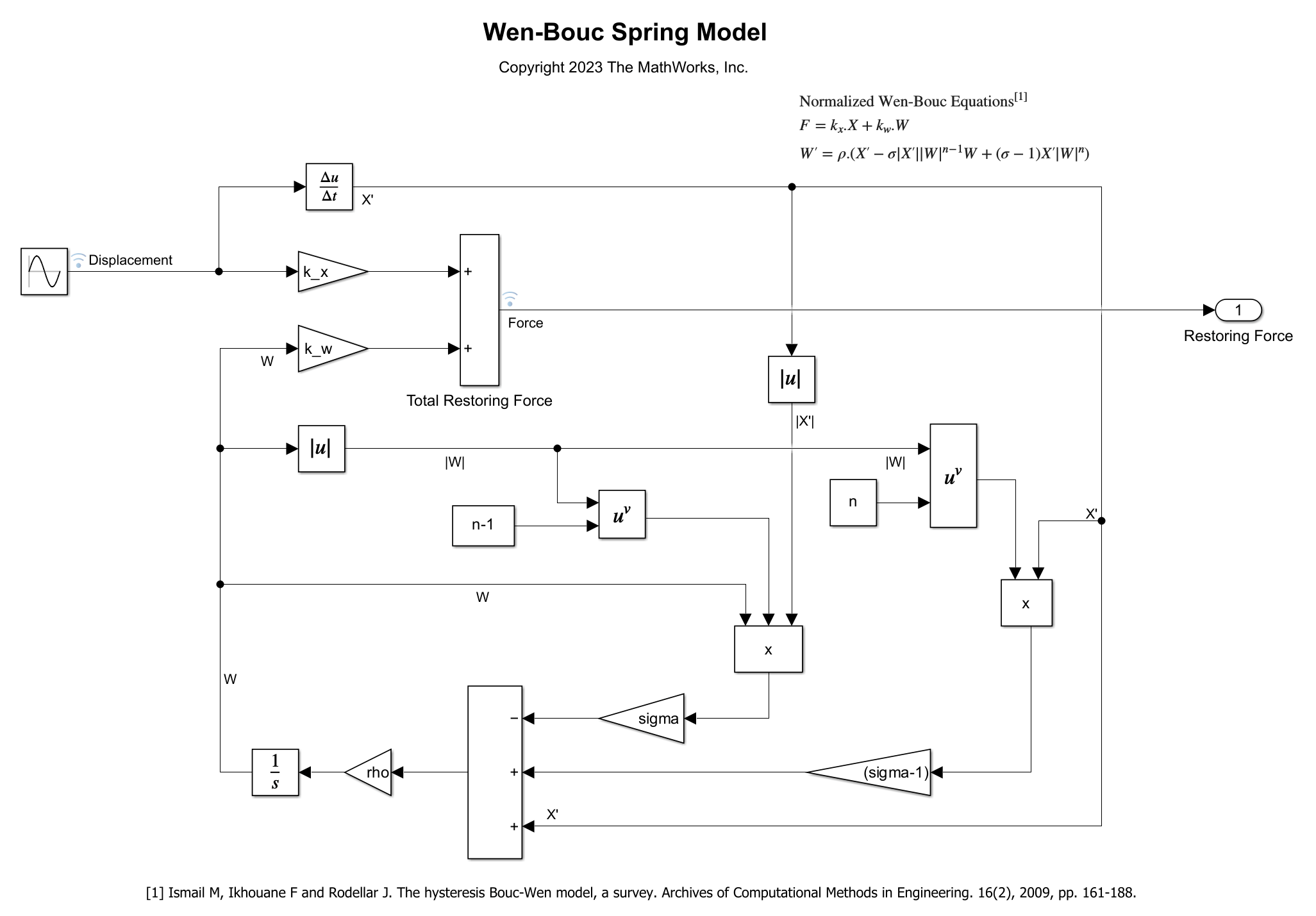

The model consists of a spring that is excited by a sine wave of Amplitude Amp. The spring's hysteresis is modeled using the normalized Wen-Bouc Hysteresis equations

$$\begin{array}{l}F=k_x.X+k_w.W\\ W^{\prime }=\rho (X^{\prime }-\sigma |X^{\prime }||W{|}^{n-1}W+(\sigma -1)X^{\prime }|W{|}^n).\end{array}$$

Here:

• $$F$$ = Restoring force exerted by the spring.

• $$X$$ = Displacement contributing to linear behavior.

• $$W$$ = Internal Displacement contributing to nonlinear behavior, with $$W_0$$ as the initial value.

• $$\rho$$, $$\sigma$$, and $$n$$ are parameters that govern the behavior of the hysteric spring.

Load Experimental Data and Define Estimation Experiment

Load the experimental data. The experimental data consists of a table ExperimentalData that contains the displacement measurements and the corresponding force measurements for the spring.

load("sdoWenBoucSpring_ExperimentalData.mat")

To link the Displacement-Force data of the table to the respective Displacement and Force signals in the model, create an experiment. Since the Displacement-Force data is not in timeseries format, create an index-based timeseries as a placeholder and store the placeholder timeseries in the value parameter of the respective signals.

Exp = sdo.Experiment(model);

Exp_Sig_Output_1 = Simulink.SimulationData.Signal;
Exp_Sig_Output_1.Name = "Displacement";
Exp_Sig_Output_1.BlockPath = strcat(model,"/Sine Wave");
Exp_Sig_Output_1.PortType = "outport";
Exp_Sig_Output_1.PortIndex = 1;
Exp_Sig_Output_1.Values = timeseries( ...
    ExperimentalData.("Displacement"), ...
    1:numel(ExperimentalData.("Displacement")));

Exp_Sig_Output_2 = Simulink.SimulationData.Signal;
Exp_Sig_Output_2.Name = "Force";
Exp_Sig_Output_2.BlockPath = strcat(model, ...
    "/Total Restoring Force");
Exp_Sig_Output_2.PortType = "outport";
Exp_Sig_Output_2.PortIndex = 1;
Exp_Sig_Output_2.Values = timeseries( ...
    ExperimentalData.("Force"), ...
    1:numel(ExperimentalData.("Force")));

Exp.OutputData = [Exp_Sig_Output_1; Exp_Sig_Output_2];

Compare Experimental Data with Initial Simulated Output

Create a simulation scenario using the experiment and obtain the initial simulated output data.

Simulator = createSimulator(Exp);
Simulator = sim(Simulator);
SimLog = find(Simulator.LoggedData, ...
    get_param(model,"SignalLoggingName"));
Force = find(SimLog,"Force");
Displacement = find(SimLog,"Displacement");

Plot the experimental and the initial simulated data.

plot(ExperimentalData.Displacement,ExperimentalData.Force,"o-",...
    Displacement.Values.Data,Force.Values.Data, ".-")
title("Responses Before Estimation")
legend("Experimental data","Simulated data", ...
    Location="northwest")

The initial model response does not match the experimental data. Therefore, use parameter estimation to tune the model parameters and match the model response to the experimental data.

Specify Parameters to Estimate

Specify the parameters to estimate, along with their minimum and maximum bounds. For example, the parameters Amp, k_w, k_x, rho, and sigma are the physical parameters that must not be negative.

p = sdo.getParameterFromModel(model, ...
    {'Amp','k_w','k_x','rho','sigma','W_0'});

p(1).Minimum = 0.94; % Amp
p(1).Maximum = 1.06; % Amp
p(2).Minimum = 0;
p(3).Minimum = 0;
p(4).Minimum = 0;
p(5).Minimum = 0;
p(6).Minimum = -1;  % W_0
p(6).Maximum = 1;   % W_0

Define Estimation Objective Function for Unconstrained Parameter Estimation

Create an objective function to evaluate how closely the model response, generated using the estimated parameter values, matches the experimental data.

The sdoWenBoucSpring_Objective function has the following input arguments:

1. The argument P that specifies the estimated parameter values.

2. The argument Exp that specifies the experiment object containing the experimental data.

3. The argument ObjectiveOptions is a structure that specifies model name, the desired type of objective cost returned (scalar or vector), and the absolute tolerance on the two signals (specified as a row vector).

The sdoWenBoucSpring_Objective function returns a structure Cost that contains the following information:

1. The error between the model response and the experimental data. This error may be returned as a scalar or a vector depending upon ObjectiveOptions.Type argument.

2. The extent to which the model response satisfies the nonzero tolerances specified in the ObjectiveOptions.AbsTol argument.

For more information on the sdoWenBoucSpring_Objective function, refer to the Supplementary Information — Objective Function section of this example.

To setup ObjectiveOptions for unconstrained optimization, set the absolute tolerances to zero and the desired error type as "vector".

ObjectiveOptions.Model = model;
ObjectiveOptions.ObjectiveCostType = "vector";
ObjectiveOptions.AbsTol = [0 0];

The sdoWenBoucSpring_Objective function requires two inputs, but sdo.optimize requires a function with one input argument. To overcome this situation, create an anonymous function OptimFcn with one input argument, P. The OptimFcn function calls sdoWenBoucSpring_Objective using two more input arguments, Exp and ObjectiveOptions.

For more information regarding anonymous functions, see Anonymous Functions.

OptimFcn = @(P) sdoWenBoucSpring_Objective(P,Exp,ObjectiveOptions);

To tune the parameter values, the optimizer callas the OptimFcn function repeatedly, until it achieves a good match between the model response and the experimental data.

Estimate parameters Using Unconstrained Parameter Estimation

Specify the optimization options. Use the nonlinear least squares (lsqnonlin) method to solve this unconstrained optimization problem.

Options = sdo.OptimizeOptions;
Options.Method = "lsqnonlin";

Use sdo.optimize function to estimate the spring parameter values.

[pOpt_Unc, info_Unc] = sdo.optimize(OptimFcn,p,Options);

 Optimization started 2024-Feb-13, 01:24:48

                                          First-order 
 Iter F-count        f(x)      Step-size  optimality
    0     13      3.52665            1
    1     26      1.12668        1.483         4.51
    2     39     0.379587       0.1736         0.82
    3     52     0.103398       0.2071        0.339
    4     65    0.0157841        1.127        0.133
    5     78   0.00627539       0.1914        0.057
    6     91   0.00051744       0.3342       0.0263
    7    104  0.000202507      0.02241       0.0229
Local minimum possible.

lsqnonlin stopped because the final change in the sum of squares relative to 
its initial value is less than the value of the function tolerance.

Compare Experimental Data with Simulated Output after Unconstrained Parameter Estimation

Update the experiments with the estimated parameter values.

Exp  = setEstimatedValues(Exp, pOpt_Unc);

Obtain the simulated output for the experiment.

Simulator = createSimulator(Exp);
Simulator = sim(Simulator);
SimLog = find(Simulator.LoggedData, ...
    get_param(model,"SignalLoggingName"));
Force = find(SimLog,"Force");
Displacement = find(SimLog,"Displacement");

Plot the experimental data and the simulated data.

plot(ExperimentalData.Displacement,ExperimentalData.Force,"o-",...
    Displacement.Values.Data,Force.Values.Data,".-")
title("Responses after Unconstrained Parameter Estimation")
legend("Experimental data","Simulated data", ...
    Location="NorthWest")

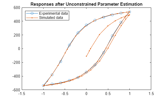
The unconstrained parameter estimation provides a good steady state fit, but the transient response of the model does not match the experimental data.

To fit the transient model response to the experimental data, perform constrained parameter estimation by specifying tolerances.

Define Estimation Objective Function for Constrained Parameter Estimation

To setup ObjectiveOptions for constrained optimization, specify the absolute tolerances as 0.06 units for Displacement and 20 units for Force. Set the desired error type to "scalar".

ObjectiveOptions.Model = model;
ObjectiveOptions.ObjectiveCostType = "scalar";
ObjectiveOptions.AbsTol = [0.06 20];

Setup OptimFcn as an anonymous function for use in sdo.optimize function.

OptimFcn = @(P) sdoWenBoucSpring_Objective(P,Exp,ObjectiveOptions);

Estimate parameters using Constrained Parameter Estimation

Use the gradient descent (fmincon) method to solve this constrained optimization problem.

Options = sdo.OptimizeOptions;
Options.Method = "fmincon";

Use sdo.optimize function to estimate the spring parameter values.

[pOpt_Con, info_Con] = sdo.optimize(OptimFcn, p, Options);

 Optimization started 2024-Feb-13, 01:26:29

                               max                     First-order 
 Iter F-count        f(x)   constraint    Step-size    optimality
    0     13      3.52665        6.392
    1     30     0.440344        5.121         1.52          225
    2     42     0.306855        4.802        0.595         1.43
    3     55    0.0112228         2.19         0.73         2.15
    4     71   0.00617541        2.039        0.119         2.49
    5     83    0.0117558        1.082        0.134        0.542
    6     95   0.00612524      0.01711       0.0749         0.16
    7    107    0.0038527            0       0.0271       0.0581
    8    119   0.00197212            0       0.0584       0.0126
    9    131   0.00179639            0       0.0214       0.0159
   10    143   0.00178618            0       0.0052         0.01
   11    155   0.00173915            0       0.0529      0.00482
   12    168   0.00172521            0       0.0256       0.0107
   13    184   0.00172479            0      0.00783       0.0117
   14    202   0.00172439            0      0.00395       0.0119
   15    211   0.00172439            0      0.00137       0.0113
Local minimum possible. Constraints satisfied.

fmincon stopped because the size of the current step is less than
the value of the step size tolerance and constraints are 
satisfied to within the value of the constraint tolerance.

Compare Experimental Data with Simulated Output after Constrained Parameter Estimation

Update the experiments with the estimated parameter values.

Exp  = setEstimatedValues(Exp,pOpt_Con);

Obtain the simulated output for the experiment.

Simulator = createSimulator(Exp);
Simulator = sim(Simulator);
SimLog = find(Simulator.LoggedData, ...
    get_param(model,"SignalLoggingName"));
Force = find(SimLog,"Force");
Displacement = find(SimLog,"Displacement");

Plot the experimental data and the simulated data.

plot(ExperimentalData.Displacement,ExperimentalData.Force,"o-",...
    Displacement.Values.Data,Force.Values.Data,".-")
title({"Responses after Constrained Parameter Estimation"})
legend("Experimental data","Simulated data", ...
    Location="NorthWest")

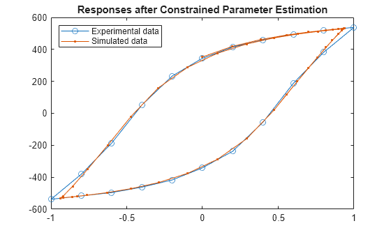
The match between the transient model response and the experimental data improves when using constrained parameter estimation.

Summary

This example demonstrates parameters estimation for scenarios where the experimental data describes correlation between two signals and is independent of time. The example achieves this time-independent parameter estimation by defining an objective function that utilizes the nearest-neighbor approach to calculate the objective cost and the tolerance cost.

The unconstrained parameter estimation demonstrates that the objective cost drives at least some portion of the model response to match the entirety of the experimental data. Additionally, the tolerance cost complements the objective cost by driving the entire model response within the specified tolerance of at least some portion of the experimental data.

You can apply the parameter estimation approach demonstrated in this example to a variety of other scenarios where time is not available as a measured variable or is not the independent variable.

Supplementary Information — Objective Function

The sdoWenBoucSpring_Objective function calculates the objective cost and the tolerance cost between the simulation output and experimental data. The function calculates the costs using the nearest neighbor approach. This approach models the experimental data as a series of reference line segments. The function then calculates the objective cost and the tolerance cost based on the distance between the simulation data points and the reference line segments.

To calculate the objective cost, the function first scales the experimental data and the simulation data. Then, it models the experimental data as a piecewise linear reference trajectory. For N number of experimental data points, the reference trajectory is composed of N-1 reference line segments. The cost vector is calculated as the distance of each reference line segment to its nearest simulation data point.

The output objective cost is a column vector with N-1 rows. However, the function converts the cost vector to a scalar, depending upon the optimization method used.

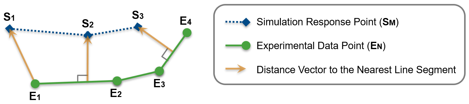
The function calculates the tolerance cost by first computing the distance vector of each simulation point from its nearest reference line segment. Then, the function determines the maximum value for each element in the distance vectors and compares it to the nonzero elements of the specified absolute tolerance. For M number of specified nonzero tolerances, the tolerance cost is a column vector with M rows.

The objective cost and the tolerance cost complement each other. The objective cost drives at least some portion of the simulation data to match the entirety of the experimental data. In contrast, the tolerance cost drives the entire simulated data to be within the specified tolerance of at least some portion of the experimental data.

To examine the estimation objective function in more detail, see the sdoWenBoucSpring_Objective.m file or use the following command.

type sdoWenBoucSpring_Objective

function Cost = sdoWenBoucSpring_Objective(P, Exp, ObjectiveOptions)
% SDOWENBOUCSPRING_OBJECTIVE This function compares model output
%                           against experimental values.
%
% Cost = sdoWenBoucSpring_Objective(P, Exp, ObjectiveOptions)
%
% The argument |P| specifies the estimated parameter values along with
% their bounds and initial values.
%
% The argument |Exp| is an object that contains the experimental data.
%
% The argument |ObjectiveOptions| is a structure that contains the model
% name, the desired type of Objective Cost returned ('scalar' or 'vector'), and the
% absolute tolerance on the two signals specified as a row vector.

% The output argument |Cost| contains information about how well the model
% simulation matches the experimental data and the information about how
% well the specified tolerances are met. The |sdo.optimize| function
% uses this information to estimate model parameters.
%
% See also sdo.optimize, sdoExampleCostFunction
%
% Copyright 2023 The MathWorks, Inc.
%%
% Update the experiment(s) with the estimated parameter values.
Exp = setEstimatedValues(Exp,P);

%% Simulate the model, and store model outputs and experimental data.
Simulator = createSimulator(Exp);
Simulator = sim(Simulator);
SimLog = find(Simulator.LoggedData, get_param(ObjectiveOptions.Model, 'SignalLoggingName'));

ExpData = [];
SimData = [];
for ctSig=1:numel(Exp.OutputData)
    Sig = find(SimLog, Exp.OutputData(ctSig).Name);
    ExpData = [ExpData, Exp.OutputData(ctSig).Values.Data];
    SimData = [SimData, Sig.Values.Data];
end

% Ensure that the experimental data is real, finite and contains two columns.  
validateattributes(ExpData, 'numeric', {'real','finite','ncols',2})

%% Return the residual errors to the optimization solver.
Cost.F = EvaluateObjectiveCost(ExpData,SimData);
if strcmp(ObjectiveOptions.ObjectiveCostType,'scalar')
    % Return the sum of square of errors as scalar.
    Cost.F = sum((Cost.F).^2);
end

% Calculate the tolerance cost if any nonzero tolerance is specified.
if any(ObjectiveOptions.AbsTol)
    Cost.Cleq = EvaluateToleranceCost(ExpData, SimData, ObjectiveOptions.AbsTol);
end
end

function ObjectiveCost = EvaluateObjectiveCost(ReferenceTrajectory, TestTrajectory)
    % EVALUATEOBJECTIVECOST Returns the residual error between reference
    %                       trajectory and test trajectory.
    %
    %   cost = EvaluateObjectiveCost([0 1;1 1],[1 1;2 -1]);
    %
    % The arguments |ReferenceTrajectory| and |TestTrajectory| are in
    % matrix form.
    %
    % The return argument |ObjectiveCost| is a column vector containing the 
    % information about how well the reference and test trajectories match.
    % data.
    % 
    % The residual is measured by considering the reference trajectory as a
    % piecewise linear curve (line segments) and computing the distance of
    % each reference line segment to its nearest test trajectory point.
    %%
    % Scale the columns of reference data by their maximum absolute values.
    [ScaledReferenceTrajectory, ScalingFactors] = MaxScale(ReferenceTrajectory);
    % Scale the columns of test data by the maximum absolute values of
    % reference data.
    ScaledTestTrajectory = TestTrajectory./ScalingFactors;
    
    % Vector to store the distances of each reference line segments.
    distances = zeros((size(ScaledReferenceTrajectory,1)-1),1);

    for index = 1:numel(distances)
        RefLineSegment = ScaledReferenceTrajectory([index, index+1],:);
        % Get distances of the line segment from all simulation points and
        % store the points on the minimum distance.
        LineDistances = arrayfun(@(i) (norm(GetDistanceFromLineSegment(RefLineSegment, ScaledTestTrajectory(i,:)))), ...
                                        (1:size(ScaledTestTrajectory,1))');
        distances(index) = min(LineDistances);
    end

    ObjectiveCost = distances; % Set the minimum distances as the cost.
end

function ToleranceCost = EvaluateToleranceCost(ReferenceTrajectory,TestTrajectory, AbsTol)
    % EVALUATETOLERANCECOST Returns the constraint cost of a test
    %                       trajectory from a reference trajectory.
    %
    %   cost = EvaluateToleranceCost([0 1;1 1],[1 1;2 -1],[0.01 0.02]);
    %
    % The arguments |ReferenceTrajectory| and |TestTrajectory| are in
    % matrix form.
    %
    % The argument |AbsTol| is a row vector specifying the tolerance values
    % for each column of the TestTrejectory.
    %
    % The return argument |ObjectiveCost| is a column vector containing the 
    % information about how well the specified tolerances are satisfied.
    %
    % The cost is calculated by considering the reference trajectory as a
    % piecewise linear curve (line segments) and computing the distance
    % components of each point on the test trajectory to the nearest
    % reference line segment. The cost is then the difference 
    % between the distance components for the farthest point and the
    % absolute tolerances.
    %%
    % Ensure the specified tolerance is a row vector with the same
    % number of columns as the reference trajectory, and contains real,
    % finite and nonnegative values. 
    validateattributes(AbsTol,'numeric', {'row','real','nonnegative','finite','ncols', size(ReferenceTrajectory,2)});

    % Row vector to store the farthest component for each dimension.
    FarthestComponents = zeros(size(AbsTol));

    for index = 1:numel(TestTrajectory(:,1))
        currentPoint = TestTrajectory(index,:);

        % Get distance vector of the test point to all reference line segments. 
        PointDistanceVectors = arrayfun(@(i) GetDistanceFromLineSegment(ReferenceTrajectory([i, i+1],:), currentPoint), ...
            (1:(size(ReferenceTrajectory,1)-1))', 'UniformOutput', false);
        PointDistanceVectors = cell2mat(PointDistanceVectors);
        PointDistances = sqrt(sum(PointDistanceVectors.^2,2));

        % Get the distance vector to the nearest reference line segment.
        [~, MinDistIndex] = min(PointDistances);
        MinDistVector = abs(PointDistanceVectors(MinDistIndex,:));

        % Update farthest value for each dimension.
        FarthestComponents = max([FarthestComponents; MinDistVector]);
    end

    % Return tolerance cost for non-zero tolerances.
    EligibleIndices = AbsTol~=0; 
    ToleranceCost = (FarthestComponents(EligibleIndices)./AbsTol(EligibleIndices))-1;
end

function DistanceVector = GetDistanceFromLineSegment(LineSegment, Point)
    % GETDISTANCEFROMLINESEGMENT Returns the distance vector of a point
    %                            from a line segment.
    %
    %   DistanceVector = GetDistanceFromLineSegment([0 1;1 1], [2 2]);
    %
    % The argument |LineSegment| is a matrix with two rows as the end
    % points of the line segment.
    %
    % The argument |Point| is a row vector with the point's coordinates.
    %
    % The output argument |DistanceVector| is a row vector that contains
    % the distance vector of the point. 
    %%
    % Ensure that the line segment is a row vector with two rows and contains
    % finite and real values.
    validateattributes(LineSegment, 'numeric', {'finite','real','nrows',2});
    % Ensure that the point is a row vector with same number of columns as
    % the line segment and contains finite and real values.
    validateattributes(Point, 'numeric', {'finite','real','row','ncols',size(LineSegment,2)});
    
    % Establish vectors of the line segment AB and the point P.
    TLineSeg = LineSegment(2,:) - LineSegment(1,:); % Vector AB
    TPoint = Point - LineSegment(1,:);  % Vector AP

    % Get length and projection of the line segment
    LSLength = norm(TLineSeg); 
    LSProjection = dot(TPoint,TLineSeg)/LSLength;

    if LSProjection <= 0
        % Projection of P falls out of the AB in direction -AB.
        DistanceVector = TPoint; % Distance is AP.

    elseif LSProjection >= LSLength
        % Projection of P falls out of the line segment in direction +AB.
        DistanceVector = TPoint-TLineSeg; % Distance is BP.

    else
        % Projection of P falls on AB then the perpendicular
        % distance of P from AB is the distance.
        DistanceVector = TPoint-(LSProjection*TLineSeg/LSLength);
    end
end

function [ScaledTrajectory, ScalingFactors] = MaxScale(Trajectory, varargin)
    % MAXSCALE Function to scale a matrix's columns by maximum absolute
    %           values or by some given values. 
    %
    %   [sTrajectory, factors] = MaxScale([0 1;2 3]);
    %   sTrajectory = MaxScale([0 1;2 3], [2 2]);
    %
    % The argument |Trajectory| is a matrix containing the trajectory values.
    %
    % An optional input argument |ScalingFactors| can be specified as a row vector.
    %
    % The output argument |ScaledTrajectory| is a matrix that contains the
    % scaled values of the trajectory.
    %
    % The output argument |ScalingFactors| is a row matric the contains the
    % scaling factors.
    %%
    if nargin==2
        % Ensure that the scaling factors are specified as a row vector
        % with same number of columns as the trajectory, and contain real,
        % finite and positive values. 
        ScalingFactors = varargin{1};
        validateattributes(ScalingFactors,'numeric',{'row','real','finite','positive', 'ncols', size(Trajectory,2)});
    else
        % Set the maximum absolute values as the scaling factors.
        ScalingFactors = max(abs(Trajectory),[],1);
        % Prevent Scaling factor = 0.
        ScalingFactors(~ScalingFactors) = 1;
    end

    ScaledTrajectory = Trajectory./ScalingFactors; % Perform scaling
end