Test Chart with Fault Detection and Redundant Logic
This example shows how to use operating points to test the response of an aircraft elevator system to an actuator failure. An operating point is a snapshot of the state of a Simulink® model during simulation. If your model contains a Stateflow® chart, the operating point includes information about active states, output and local data, and persistent variables. For more information, see Save and Restore Operating Points for Stateflow Charts.
The model sf_aircraft demonstrates a fault detection, isolation, and
recovery (FDIR) application for a pair of aircraft elevators controlled by redundant
actuators.

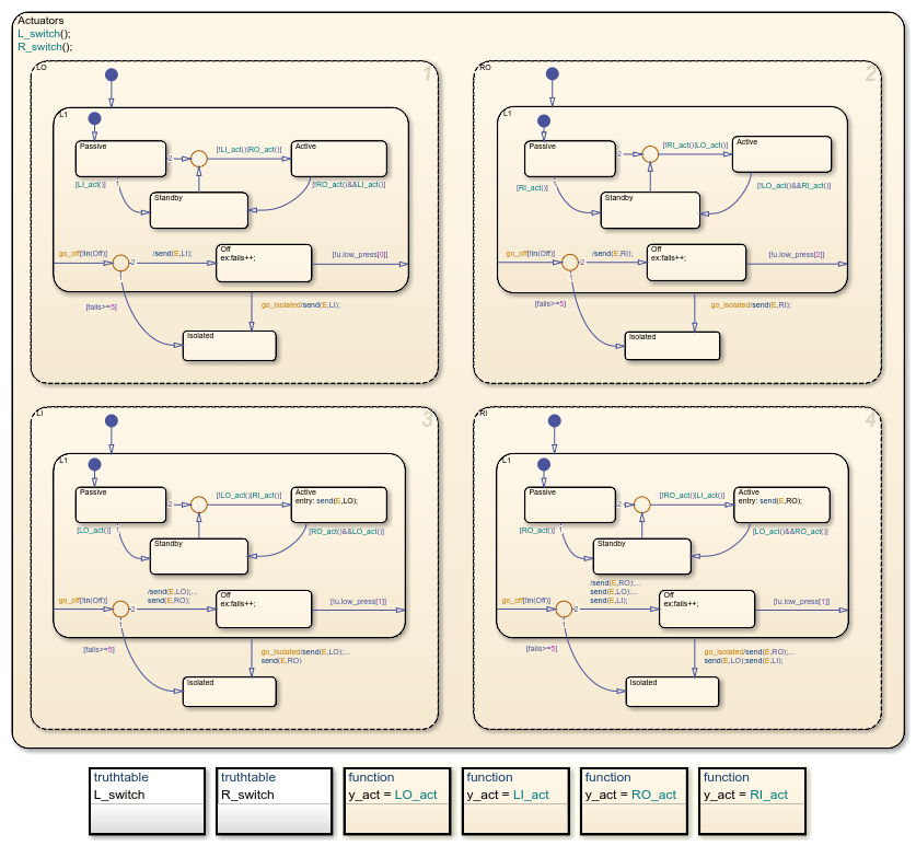
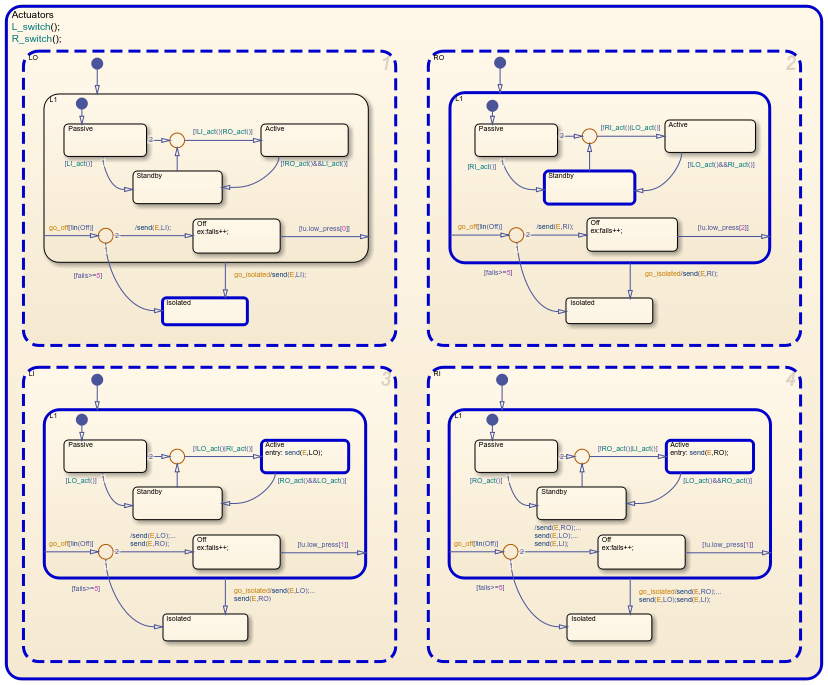
The Mode Logic chart monitors the status of the four actuators. Each
elevator has a primary, outer actuator (represented by the states LO and
RO) and a secondary, inner actuator (represented by the states
LI and RI). In normal operation, the outer actuators
are active and the inner actuators are on standby.
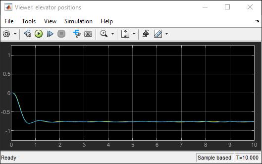
When the actuators work correctly, the left and right elevators reach steady-state positions in 3 seconds.
To see what happens when one actuator fails, you can simulate the model, save the operating point at t = 3, modify the operating point to reflect an actuator failure, and then simulate again between t = 3 and t = 10.
For more information about this model, see Detect Faults in Aircraft Elevator Control System.
Define Operating Point for Steady State
Open the
sf_aircraftmodel.openExample("sf_aircraft")Set the model to save the final operating point. Open the Configuration Parameters dialog box and, in the Data Import/Export pane:
Select Final states and enter a name for the operating point. For this example, use
xSteadyState.Select Save final operating point.
Click OK.
Set the stop time for this simulation segment. In the Simulation tab, set Stop Time to
3.Run the simulation.
When you simulate the model, you save the final operating point at t = 3 in the variable
xSteadyStatein the MATLAB® base workspace.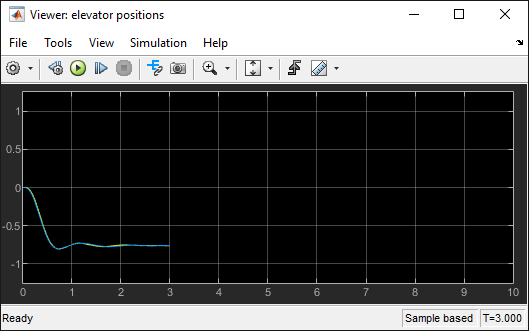
In the Configuration Parameters dialog box, in the Data Import/Export pane, clear the Save final operating point and Final states parameters. This step prevents you from overwriting the operating point you saved in the previous step.
Modify Operating Point Values for Actuator Failure
Access the
Stateflow.op.BlockOperatingPointobject that contains the operating point information for theMode Logicchart.blockpath = "sf_aircraft/Mode Logic"; op = get(xSteadyState,blockpath)op = Block: "Mode Logic" (handle) (active) Path: sf_aircraft/Mode Logic Contains: + Actuators "State (OR)" (active) + LI_act "Function" + LO_act "Function" + L_switch "Function" + RI_act "Function" + RO_act "Function" + R_switch "Function" LI_mode "State output data" sf_aircraft_ModeType [1,1] LO_mode "State output data" sf_aircraft_ModeType [1,1] RI_mode "State output data" sf_aircraft_ModeType [1,1] RO_mode "State output data" sf_aircraft_ModeType [1,1]The operating point contains a list of states, functions, and data in hierarchical order.
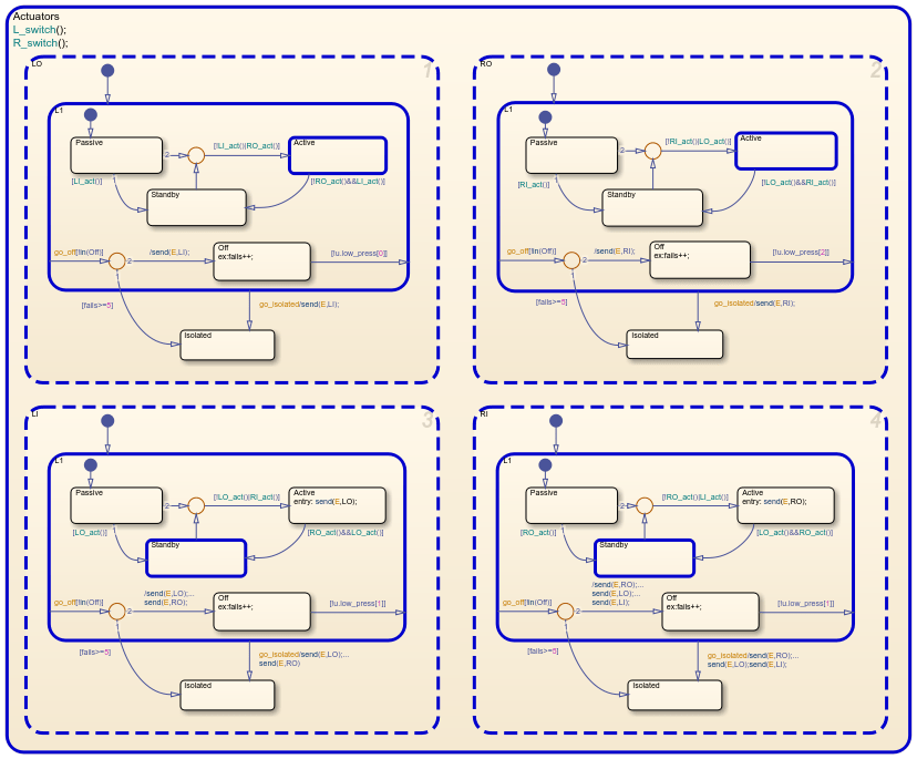
Highlight the states that are active in your chart at t = 3.
highlightActiveStates(op)
Active states appear highlighted. The two outer actuators are active and the two inner actuators are on standby.
Change the substate activity in the state
LOto reflect a failure of the left-outer actuator.setActive(op.Actuators.LO.Isolated)

Note
The
setActivefunction ensures that the chart exits and enters the appropriate states to maintain state consistency. However, the method does not performexitactions for the previously active substate orentryactions for the newly active substate.Save the modified operating point as the workspace variable
xFailure.xFailure = set(xSteadyState,blockpath,op);
Test Model Behavior after Actuator Failure
Load the operating point as the initial state of the model. In the Configuration Parameters dialog box, in the Data Import/Export pane, select Initial state and enter the variable that contains the modified operating point of your chart,
xFailure. Then, click OK.Define the stop time for the simulation segment to test. In the Simulation tab, set Stop Time to
10.Run the simulation.
The chart animation shows how the other three actuators react to the failure of the left-outer actuator:
The left-inner actuator switches from standby to active to compensate for the left-outer actuator failure.
The right-inner actuator switches from standby to active because the same hydraulic line connects to both inner actuators.
The right-outer actuator switches from active to standby because only one actuator can be active for each elevator.
After the failure, both elevators continue to maintain steady-state positions.

See Also
Model Settings
- Initial state (Simulink) | Final states (Simulink) | Save final operating point (Simulink)
Objects
Stateflow.op.BlockOperatingPoint|Stateflow.op.OperatingPointContainer|Stateflow.op.OperatingPointData
Functions
highlightActiveStates|setActive|get(Simulink) |set(Simulink)
Related Topics
You can also select a web site from the following list:
Americas
- América Latina (Español)
- Canada (English)
- United States (English)
Europe
- Belgium (English)
- Denmark (English)
- Deutschland (Deutsch)
- España (Español)
- Finland (English)
- France (Français)
- Ireland (English)
- Italia (Italiano)
- Luxembourg (English)
- Netherlands (English)
- Norway (English)
- Österreich (Deutsch)
- Portugal (English)
- Sweden (English)
- Switzerland
- United Kingdom (English)