Choose Model Options In Regression Learner
Choose Regression Model Type
You can use the Regression Learner app to automatically train a selection of different models on your data. Use automated training to quickly try a selection of model types, and then explore promising models interactively. To get started, try these options first:

| Get Started Regression Model Options | Description |
|---|---|
| All Quick-To-Train | Try the All Quick-To-Train option first. The app trains all model types that are typically quick to train. |
| All | Use the All option to train all available nonoptimizable model types. Trains every type regardless of any prior trained models. Can be time-consuming. |
To learn more about automated model training, see Automated Regression Model Training.
If you want to explore models one at a time, or if you already know what model type you want, you can select individual models or train a group of the same type. To see all available regression model options, on the Learn tab, click the arrow in the Models section to expand the list of regression models. The nonoptimizable model options in the gallery are preset starting points with different settings, suitable for a range of different regression problems. To use optimizable model options and tune model hyperparameters automatically, see Hyperparameter Optimization in Regression Learner App.
For help choosing the best model type for your problem, see the tables showing typical characteristics of different supervised learning algorithms and the MATLAB® function called by each one. Decide on the tradeoff you want in speed, flexibility, and interpretability. The best model type depends on your data.
Tip
To avoid overfitting, look for a less flexible model that provides sufficient accuracy. For example, look for simple models such as regression trees that are fast and easy to interpret. If the models are not accurate enough predicting the response, choose other models with higher flexibility, such as ensembles. To control flexibility, see the details for each model type.
Characteristics of Regression Model Types
| Regression Model Type | Interpretability | Function |
|---|---|---|
| Linear Regression Models | Easy | fitlm |
| Regression Trees | Easy | fitrtree |
| Support Vector Machines | Easy for linear SVMs. Hard for other kernels. | fitrsvm |
| Efficiently Trained Linear Regression Models | Easy | fitrlinear |
| Gaussian Process Regression Models | Hard | fitrgp |
| Kernel Approximation Models | Hard | fitrkernel |
| Ensembles of Trees | Hard | fitrensemble |
| Neural Networks | Hard | fitrnet |
| Customizable Neural Network Models | Hard | fitrnet (with Network
argument) |
To read a description of each model in Regression Learner, switch to the details view in the list of all model presets.

Tip
The nonoptimizable models in the Models gallery are preset starting points with different settings. After you choose a model type, such as regression trees, try training all the nonoptimizable presets to see which one produces the best model with your data.
For workflow instructions, see Train Regression Models in Regression Learner App.
Categorical Predictor Support
In Regression Learner, all model types support categorical predictors.
Tip
If you have categorical predictors with many unique values, training linear models with interaction or quadratic terms and stepwise linear models can use a lot of memory. If the model fails to train, try removing these categorical predictors.
Linear Regression Models
Linear regression models have predictors that are linear in the model parameters, are easy to interpret, and are fast for making predictions. These characteristics make linear regression models popular models to try first. However, the highly constrained form of these models means that they often have low predictive accuracy. After fitting a linear regression model, try creating more flexible models, such as regression trees, and compare the results.
Tip
In the Models gallery, click All Linear to try each of the linear regression options and see which settings produce the best model with your data. Select the best model in the Models pane and try to improve that model by using feature selection and changing some advanced options.
| Regression Model Type | Interpretability | Model Flexibility |
|---|---|---|
| Linear | Easy | Very low |
| Interactions Linear | Easy | Medium |
| Robust Linear | Easy | Very low. Less sensitive to outliers, but might be slow to train. |
| Stepwise Linear | Easy | Medium |
For a workflow example, see Train Regression Trees Using Regression Learner App.
Linear Regression Model Hyperparameter Options
Regression Learner uses the fitlm function to train Linear,
Interactions Linear, and Robust Linear models. The app uses the stepwiselm function to train
Stepwise Linear models.
For Linear, Interactions Linear, and Robust Linear models you can set these options:
Terms
Specify which terms to use in the linear model. You can choose from:
Linear. A constant term and linear terms in the predictorsInteractions. A constant term, linear terms, and interaction terms between the predictorsPure Quadratic. A constant term, linear terms, and terms that are purely quadratic in each of the predictorsQuadratic. A constant term, linear terms, and quadratic terms (including interactions)
Robust option
Specify whether to use a robust objective function and make your model less sensitive to outliers. With this option, the fitting method automatically assigns lower weights to data points that are more likely to be outliers.
Stepwise linear regression starts with an initial model and systematically adds and removes terms to the model based on the explanatory power of these incrementally larger and smaller models. For Stepwise Linear models, you can set these options:
Initial terms
Specify the terms that are included in the initial model of the stepwise procedure. You can choose from
Constant,Linear,Interactions,Pure Quadratic, andQuadratic.Upper bound on terms
Specify the highest order of the terms that the stepwise procedure can add to the model. You can choose from
Linear,Interactions,Pure Quadratic, andQuadratic.Maximum number of steps
Specify the maximum number of different linear models that can be tried in the stepwise procedure. To speed up training, try reducing the maximum number of steps. Selecting a small maximum number of steps decreases your chances of finding a good model.
Tip
If you have categorical predictors with many unique values, training linear models with interaction or quadratic terms and stepwise linear models can use a lot of memory. If the model fails to train, try removing these categorical predictors.
Regression Trees
Regression trees are easy to interpret, fast for fitting and prediction, and low on memory usage. Try to grow smaller trees with fewer larger leaves to prevent overfitting. Control the leaf size with the Minimum leaf size setting.
Tip
In the Models gallery, click All Trees to try each of the nonoptimizable regression tree options and see which settings produce the best model with your data. Select the best model in the Models pane, and try to improve that model by using feature selection and changing some advanced options.
| Regression Model Type | Interpretability | Model Flexibility |
|---|---|---|
| Fine Tree | Easy | High Many small leaves for a highly flexible response function (Minimum leaf size is 4.) |
| Medium Tree | Easy | Medium Medium-sized leaves for a less flexible response function (Minimum leaf size is 12.) |
| Coarse Tree | Easy | Low Few large leaves for a coarse response function (Minimum leaf size is 36.) |
To predict a response of a regression tree, follow the tree from the root (beginning) node down to a leaf node. The leaf node contains the value of the response.
Statistics and Machine Learning Toolbox™ trees are binary. Each step in a prediction involves checking the value of one predictor variable. For example, here is a simple regression tree

This tree predicts the response based on two predictors, x1 and
x2. To make a prediction, start at the top node. At each
node, check the values of the predictors to decide which branch to follow. When the
branches reach a leaf node, the response is set to the value corresponding to that
node.
You can visualize your regression tree model by exporting the model from the app, and then entering:
view(trainedModel.RegressionTree,"Mode","graph")
For a workflow example, see Train Regression Trees Using Regression Learner App.
Regression Tree Model Hyperparameter Options
The Regression Learner app uses the fitrtree function to train
regression trees. You can set these options:
Minimum leaf size
Specify the minimum number of training samples used to calculate the response of each leaf node. When you grow a regression tree, consider its simplicity and predictive power. To change the minimum leaf size, click the buttons or enter a positive integer value in the Minimum leaf size box.
A fine tree with many small leaves is usually highly accurate on the training data. However, the tree might not show comparable accuracy on an independent test set. A very leafy tree tends to overfit, and its validation accuracy is often far lower than its training (or resubstitution) accuracy.
In contrast, a coarse tree with fewer large leaves does not attain high training accuracy. But a coarse tree can be more robust in that its training accuracy can be near that of a representative test set.
Tip
Decrease the Minimum leaf size to create a more flexible model.
Surrogate decision splits — For missing data only.
Specify surrogate use for decision splits. If you have data with missing values, use surrogate splits to improve the accuracy of predictions.
When you set Surrogate decision splits to
On, the regression tree finds at most 10 surrogate splits at each branch node. To change the number of surrogate splits, click the buttons or enter a positive integer value in the Maximum surrogates per node box.When you set Surrogate decision splits to
Find All, the regression tree finds all surrogate splits at each branch node. TheFind Allsetting can use considerable time and memory.
Alternatively, you can let the app choose some of these model options automatically by using hyperparameter optimization. See Hyperparameter Optimization in Regression Learner App.
Support Vector Machines
You can train regression support vector machines (SVMs) in Regression Learner. Linear SVMs are easy to interpret, but can have low predictive accuracy. Nonlinear SVMs are more difficult to interpret, but can be more accurate.
Tip
In the Models gallery, click All SVMs to try each of the nonoptimizable SVM options and see which settings produce the best model with your data. Select the best model in the Models pane, and try to improve that model by using feature selection and changing some advanced options.
| Regression Model Type | Interpretability | Model Flexibility |
|---|---|---|
| Linear SVM | Easy | Low |
| Quadratic SVM | Hard | Medium |
| Cubic SVM | Hard | Medium |
| Fine Gaussian SVM | Hard | High Allows rapid variations in the response function. Kernel scale is set to sqrt(P)/4, where
P is the number of predictors. |
| Medium Gaussian SVM | Hard | Medium Gives a less flexible response function. Kernel scale is set to sqrt(P). |
| Coarse Gaussian SVM | Hard | Low Gives a rigid response function. Kernel scale is set to sqrt(P)*4. |
Statistics and Machine Learning Toolbox implements linear epsilon-insensitive SVM regression. This SVM ignores prediction errors that are less than some fixed number ε. The support vectors are the data points that have errors larger than ε. The function the SVM uses to predict new values depends only on the support vectors. To learn more about SVM regression, see Understanding Support Vector Machine Regression.
For a workflow example, see Train Regression Trees Using Regression Learner App.
SVM Model Hyperparameter Options
Regression Learner uses the fitrsvm function to train SVM
regression models.
You can set these options in the app:
Kernel function
The kernel function determines the nonlinear transformation applied to the data before the SVM is trained. You can choose from:
Gaussianor Radial Basis Function (RBF) kernelLinearkernel, easiest to interpretQuadratickernelCubickernel
Box constraint mode
The box constraint controls the penalty imposed on observations with large residuals. A larger box constraint gives a more flexible model. A smaller value gives a more rigid model, less sensitive to overfitting.
When Box constraint mode is set to
Auto, the app uses a heuristic procedure to select the box constraint when the kernel function isGaussian. For all other kernel functions, the app sets the box constraint equal to1. For more information, see theBoxConstraintname-value argument offitrsvm.Try to fine-tune your model by specifying the box constraint manually. Set Box constraint mode to
Manualand specify a value. Change the value by clicking the arrows or entering a positive scalar value in the Manual box constraint box. The app automatically preselects a reasonable value for you. Try to increase or decrease this value slightly and see if this improves your model.Tip
Increase the box constraint value to create a more flexible model.
Epsilon mode
Prediction errors that are smaller than the epsilon (ε) value are ignored and treated as equal to zero. A smaller epsilon value gives a more flexible model.
When Epsilon mode is set to
Auto, the app uses a heuristic procedure to select the kernel scale.Try to fine-tune your model by specifying the epsilon value manually. Set Epsilon mode to
Manualand specify a value. Change the value by clicking the arrows or entering a positive scalar value in the Manual epsilon box. The app automatically preselects a reasonable value for you. Try to increase or decrease this value slightly and see if this improves your model.Tip
Decrease the epsilon value to create a more flexible model.
Kernel scale mode
The kernel scale controls the scale of the predictors on which the kernel varies significantly. A smaller kernel scale gives a more flexible model.
When Kernel scale mode is set to
Auto, the app uses a heuristic procedure to select the kernel scale.Try to fine-tune your model by specifying the kernel scale manually. Set Kernel scale mode to
Manualand specify a value. Change the value by clicking the arrows or entering a positive scalar value in the Manual kernel scale box. The app automatically preselects a reasonable value for you. Try to increase or decrease this value slightly and see if this improves your model.Tip
Decrease the kernel scale value to create a more flexible model.
Standardize data
Standardizing the predictors transforms them so that they have mean 0 and standard deviation 1. Standardizing removes the dependence on arbitrary scales in the predictors and generally improves performance.
Alternatively, you can let the app choose some of these model options automatically by using hyperparameter optimization. See Hyperparameter Optimization in Regression Learner App.
Efficiently Trained Linear Regression Models
The efficiently trained linear regression models use techniques that reduce the training computation time at the cost of some accuracy. The available efficiently trained models are linear least-squares models and linear support vector machines (SVMs). When training on data with many predictors or many observations, consider using efficiently trained linear regression models instead of the existing linear or linear SVM preset models.
Tip
In the Models gallery, click All Efficiently Trained Linear Models to try each of the preset efficient linear model options and see which settings produce the best model with your data. Select the best model in the Models pane, and try to improve that model by using feature selection and changing some advanced options.
| Regression Model Type | Interpretability | Model Flexibility |
|---|---|---|
| Efficient Linear Least Squares | Easy | Medium — increases as the Beta tolerance setting decreases |
| Efficient Linear SVM | Easy | Medium — increases as the Beta tolerance setting decreases |
For an example, see Compare Linear Regression Models Using Regression Learner App.
Efficiently Trained Linear Model Hyperparameter Options
Regression Learner uses the fitrlinear function to create
efficiently trained linear regression models. You can set the following options:
Learner — Specify the learner type for the efficient linear regression model, either
SVMorLeast squares. SVM models use an epsilon-insensitive loss during model fitting, whereas least-squares models use a mean squared error (MSE). For more information, seeLearner.Solver — Specify the objective function minimization technique to use for training. Depending on your data and the other hyperparameter values, the available solver options are
SGD,ASGD,Dual SGD,BFGS,LBFGS,SpaRSA, andAuto.When you set this option to
Auto, the software selects:BFGS when the data contains 100 or fewer predictor variables and the model uses a ridge penalty
SpaRSA when the data contains 100 or fewer predictor variables and the model uses a lasso penalty
Dual SGD when the data contains more than 100 predictor variables and the model uses an SVM learner with a ridge penalty
SGD otherwise
For more information, see
Solver.Regularization — Specify the complexity penalty type, either a lasso (L1) penalty or a ridge (L2) penalty. Depending on the other hyperparameter values, the available regularization options are
Lasso,Ridge, andAuto.When you set this option to
Auto, the software selects:Lasso when the model uses a SpaRSA solver
Ridge otherwise
For more information, see
Regularization.Regularization strength (Lambda) — Specify lambda, the regularization strength.
When you set this option to
Auto, the software sets the regularization strength to 1/n, where n is the number of observations.When you set this option to
Manual, you can specify a value by clicking the arrows or entering a positive scalar value in the box.
For more information, see
Lambda.Relative coefficient tolerance (Beta tolerance) — Specify the beta tolerance, which is the relative tolerance on the linear coefficients and bias term (intercept). The beta tolerance affects when the training process ends. If the software converges too quickly to a model that performs poorly, you can decrease the beta tolerance to try to improve the fit. The default value is 0.0001. For more information, see
BetaTolerance.Epsilon — Specify half the width of the epsilon-insensitive band. This option is available when Learner is
SVM.When you set this option to
Auto, the software determines the value of Epsilon asiqr(Y)/13.49, which is an estimate of a tenth of the standard deviation using the interquartile range of the response variableY. Ifiqr(Y)is equal to zero, then the software sets the value to 0.1.When you set this option to
Manual, you can specify a value by clicking the arrows or entering a positive scalar value in the box.
For more information, see
Epsilon.
Alternatively, you can let the app choose some of these model options automatically by using hyperparameter optimization. See Hyperparameter Optimization in Regression Learner App.
Gaussian Process Regression Models
You can train Gaussian process regression (GPR) models in Regression Learner. GPR models are often highly accurate, but can be difficult to interpret.
Tip
In the Models gallery, click All GPR Models to try each of the nonoptimizable GPR model options and see which settings produce the best model with your data. Select the best model in the Models pane, and try to improve that model by using feature selection and changing some advanced options.
| Regression Model Type | Interpretability | Model Flexibility |
|---|---|---|
| Rational Quadratic | Hard | Automatic |
| Squared Exponential | Hard | Automatic |
| Matern 5/2 | Hard | Automatic |
| Exponential | Hard | Automatic |
In Gaussian process regression, the response is modeled using a probability distribution over a space of functions. The flexibility of the presets in the Models gallery is automatically chosen to give a small training error and, simultaneously, protection against overfitting. To learn more about Gaussian process regression, see Gaussian Process Regression Models.
For a workflow example, see Train Regression Trees Using Regression Learner App.
Gaussian Process Regression Model Hyperparameter Options
Regression Learner uses the fitrgp function to train GPR
models.
You can set these options in the app:
Basis function
The basis function specifies the form of the prior mean function of the Gaussian process regression model. You can choose from
Zero,Constant, andLinear. Try to choose a different basis function and see if this improves your model.Kernel function
The kernel function determines the correlation in the response as a function of the distance between the predictor values. You can choose from
Rational Quadratic,Squared Exponential,Matern 5/2,Matern 3/2, andExponential.To learn more about kernel functions, see Kernel (Covariance) Function Options.
Use isotropic kernel
If you use an isotropic kernel, the correlation length scales are the same for all the predictors. With a nonisotropic kernel, each predictor variable has its own separate correlation length scale.
Using a nonisotropic kernel can improve the accuracy of your model, but can make the model slow to fit.
To learn more about nonisotropic kernels, see Kernel (Covariance) Function Options.
Kernel mode
You can manually specify initial values of the kernel parameters Kernel scale and Signal standard deviation. The signal standard deviation is the prior standard deviation of the response values. By default the app locally optimizes the kernel parameters starting from the initial values. To use fixed kernel parameters, set Optimize numeric parameters to
No.When Kernel scale mode is set to
Auto, the app uses a heuristic procedure to select the initial kernel parameters.If you set Kernel scale mode to
Manual, you can specify the initial values. Click the buttons or enter a positive scalar value in the Kernel scale box and the Signal standard deviation box.If you set Use isotropic kernel to
No, you cannot set initial kernel parameters manually.Sigma mode
You can specify manually the initial value of the observation noise standard deviation Sigma. By default the app optimizes the observation noise standard deviation, starting from the initial value. To use fixed kernel parameters, clear the Optimize numeric parameters check box in the advanced options.
When Sigma mode is set to
Auto, the app uses a heuristic procedure to select the initial observation noise standard deviation.If you set Sigma mode to
Manual, you can specify the initial values. Click the buttons or enter a positive scalar value in the Sigma box.Standardize data
Standardizing the predictors transforms them so that they have mean 0 and standard deviation 1. Standardizing removes the dependence on arbitrary scales in the predictors and generally improves performance.
Optimize numeric parameters
With this option, the app automatically optimizes numeric parameters of the GPR model. The optimized parameters are the coefficients of the Basis function, the kernel parameters Kernel scale and Signal standard deviation, and the observation noise standard deviation Sigma.
Alternatively, you can let the app choose some of these model options automatically by using hyperparameter optimization. See Hyperparameter Optimization in Regression Learner App.
Kernel Approximation Models
In Regression Learner, you can use kernel approximation models to perform nonlinear regression of data with many observations. For large in-memory data, kernel approximation models tend to train and predict faster than SVM models with Gaussian kernels.
Gaussian kernel regression models map predictors in a low-dimensional space into a high-dimensional space, and then fit a linear model to the transformed predictors in the high-dimensional space. Choose between fitting an SVM linear model and fitting a least-squares linear model in the expanded space.
Tip
In the Models gallery, click All Kernels to try each of the preset kernel approximation options and see which settings produce the best model with your data. Select the best model in the Models pane, and try to improve that model by using feature selection and changing some advanced options.
| Regression Model Type | Interpretability | Model Flexibility |
|---|---|---|
| SVM Kernel | Hard | Medium — increases as the Kernel scale setting decreases |
| Least Squares Kernel Regression | Hard | Medium — increases as the Kernel scale setting decreases |
Kernel Model Hyperparameter Options
Regression Learner uses the fitrkernel function to train kernel approximation regression
models.
You can set these options on the Summary tab for the selected model:
Learner — Specify the linear regression model type to fit in the expanded space, either
SVMorLeast Squares Kernel. SVM models use an epsilon-insensitive loss during model fitting, whereas least-square models use a mean squared error (MSE).Number of expansion dimensions — Specify the number of dimensions in the expanded space.
When you set this option to
Auto, the software sets the number of dimensions to2.^ceil(min(log2(p)+5,15)), wherepis the number of predictors.When you set this option to
Manual, you can specify a value by clicking the arrows or entering a positive scalar value in the box.
Regularization strength (Lambda) — Specify the ridge (L2) regularization penalty term. When you use an SVM learner, the box constraint C and the regularization term strength λ are related by C = 1/(λn), where n is the number of observations.
When you set this option to
Auto, the software sets the regularization strength to 1/n, where n is the number of observations.When you set this option to
Manual, you can specify a value by clicking the arrows or entering a positive scalar value in the box.
Kernel scale — Specify the kernel scaling. The software uses this value to obtain a random basis for the random feature expansion. For more details, see Random Feature Expansion.
When you set this option to
Auto, the software uses a heuristic procedure to select the scale value. The heuristic procedure uses subsampling. Therefore, to reproduce results, set a random number seed usingrngbefore training the regression model.When you set this option to
Manual, you can specify a value by clicking the arrows or entering a positive scalar value in the box.
Epsilon — Specify half the width of the epsilon-insensitive band. This option is available when Learner is
SVM.When you set this option to
Auto, the software determines the value of Epsilon asiqr(Y)/13.49, which is an estimate of a tenth of the standard deviation using the interquartile range of the response variableY. Ifiqr(Y)is equal to zero, then the software sets the value to 0.1.When you set this option to
Manual, you can specify a value by clicking the arrows or entering a positive scalar value in the box.
Standardize data — Specify whether to standardize the numeric predictors. If predictors have widely different scales, standardizing can improve the fit.
Iteration limit — Specify the maximum number of training iterations.
Alternatively, you can let the app choose some of these model options automatically by using hyperparameter optimization. See Hyperparameter Optimization in Regression Learner App.
Ensembles of Trees
You can train ensembles of regression trees in Regression Learner. Ensemble models combine results from many weak learners into one high-quality ensemble model.
Tip
In the Models gallery, click All Ensembles to try each of the nonoptimizable ensemble options and see which settings produce the best model with your data. Select the best model in the Models pane, and try to improve that model by using feature selection and changing some advanced options.
| Regression Model Type | Interpretability | Ensemble Method | Model Flexibility |
|---|---|---|---|
| Boosted Trees | Hard | Least-squares boosting ( | Medium to high |
| Bagged Trees | Hard | Bootstrap aggregating or bagging, with regression tree learners. | High |
For a workflow example, see Train Regression Trees Using Regression Learner App.
Ensemble Model Hyperparameter Options
Regression Learner uses the fitrensemble function to train
ensemble models. You can set these options:
Minimum leaf size
Specify the minimum number of training samples used to calculate the response of each leaf node. When you grow a regression tree, consider its simplicity and predictive power. To change the minimum leaf size, click the buttons or enter a positive integer value in the Minimum leaf size box.
A fine tree with many small leaves is usually highly accurate on the training data. However, the tree might not show comparable accuracy on an independent test set. A very leafy tree tends to overfit, and its validation accuracy is often far lower than its training (or resubstitution) accuracy.
In contrast, a coarse tree with fewer large leaves does not attain high training accuracy. But a coarse tree can be more robust in that its training accuracy can be near that of a representative test set.
Tip
Decrease the Minimum leaf size to create a more flexible model.
Number of learners
Try changing the number of learners to see if you can improve the model. Many learners can produce high accuracy, but can be time consuming to fit.
Tip
Increase the Number of learners to create a more flexible model.
Learning rate
For boosted trees, specify the learning rate for shrinkage. If you set the learning rate to less than 1, the ensemble requires more learning iterations but often achieves better accuracy. 0.1 is a popular initial choice.
Number of predictors to sample
Specify the number of predictors to select at random for each split in the tree learners.
When you select the
Auto(default) option for a Bagged Tree model, the software uses one third of the number of predictors. For a Boosted Tree model, theAutooption is equivalent toSelect All. For more information, see theNumVariablesToSampleargument oftemplateTree.When you select
Select All, the software uses all available predictors.When you select
Set Limit, you can specify a value by clicking the arrows or entering a positive integer value in the box.
Alternatively, you can let the app choose some of these model options automatically by using hyperparameter optimization. See Hyperparameter Optimization in Regression Learner App.
Neural Networks
Neural network models typically have good predictive accuracy; however, they are not easy to interpret.
Model flexibility increases with the size and number of fully connected layers in the neural network.
Tip
In the Models gallery, click All Simple Neural Networks to try each of the preset neural network options and see which settings produce the best model with your data. Select the best model in the Models pane, and try to improve that model by using feature selection and changing some advanced options.
If you have a Deep Learning Toolbox™ license, you can select additional presets for fully customizable neural network models. For more information, see Customizable Neural Network Models.
| Regression Model Type | Interpretability | Model Flexibility |
|---|---|---|
| Narrow Neural Network | Hard | Medium — increases with the First layer size setting |
| Medium Neural Network | Hard | Medium — increases with the First layer size setting |
| Wide Neural Network | Hard | Medium — increases with the First layer size setting |
| Bilayered Neural Network | Hard | High — increases with the First layer size and Second layer size settings |
| Trilayered Neural Network | Hard | High — increases with the First layer size, Second layer size, and Third layer size settings |
Each model is a feedforward, fully connected neural network for regression. The first fully connected layer of the neural network has a connection from the network input (predictor data), and each subsequent layer has a connection from the previous layer. Each fully connected layer multiplies the input by a weight matrix and then adds a bias vector. An activation function follows each fully connected layer, excluding the last. The final fully connected layer produces the network's output, namely predicted response values. For more information, see Neural Network Structure.
After you train a neural network model, you can display its network architecture and layer information. In the Plots and Results section of the Learn tab, click the arrow to open the gallery, and then click Analyze Network in the Neural Network Results group. This option is also available in the Network Architecture section of the Summary tab.
The app displays information about each layer in the network. For more
information about neural network layers, see the fitrnet function page and the topic List of Deep Learning Layers (Deep Learning Toolbox).

Neural Network Model Hyperparameter Options
Regression Learner uses the fitrnet function to train neural network models. You can set
these options:
Number of fully connected layers — Specify the number of fully connected layers in the neural network, excluding the final fully connected layer for regression. You can choose a maximum of three fully connected layers. If you require a network with more layers and have a Deep Learning Toolbox license, see Customizable Neural Network Models.
First layer size, Second layer size, and Third layer size — Specify the size of each fully connected layer, excluding the final fully connected layer. If you choose to create a neural network with multiple fully connected layers, consider specifying layers with decreasing sizes.
Activation — Specify the activation function for all fully connected layers, excluding the final fully connected layer. Choose from the following activation functions:
ReLU,Tanh,None, andSigmoid.Iteration limit — Specify the maximum number of training iterations.
Regularization strength (Lambda) — Specify the ridge (L2) regularization penalty term.
Standardize data — Specify whether to standardize the numeric predictors. If predictors have widely different scales, standardizing can improve the fit. Standardizing the data is highly recommended.
Alternatively, you can let the app choose some of these model options automatically by using hyperparameter optimization. See Hyperparameter Optimization in Regression Learner App.
View Training Progress Plots for Neural Network
After you train a regular or customizable neural network model, you can view plots that show how the training progressed. In the Plots and Results section, click the arrow to open the gallery, and then click Training Progress in the Neural Network Results group.
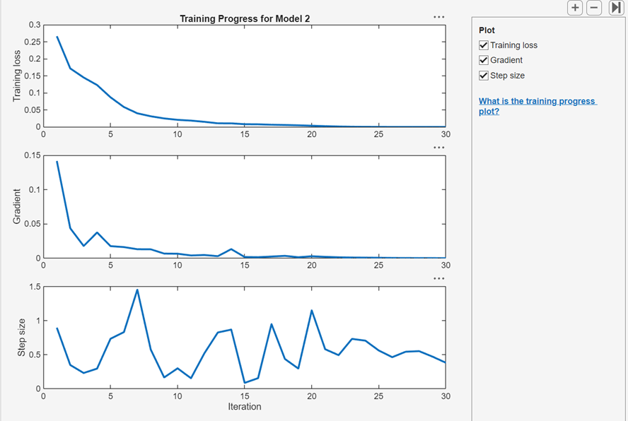
In the Plot pane, you can select check boxes to display
the cross-entropy training loss, optimization gradient, and step size values at
each training iteration. You can use these plots to assess model optimization
convergence and to check for possible overfitting. For more information about
neural network training parameters, see the fitrnet function page.
Customizable Neural Network Models
Since R2026a
If you have a Deep Learning Toolbox license, you can select two additional presets for neural network models:
Fully connected customizable neural network — A customizable fully connected network that is similar to the Bilayered and Trilayered Neural Network presets, but has five fully connected layers.
Residual customizable neural network — A customizable network that contains one residual connection. Residual connections improve gradient flow through the network and enable you to train deeper networks.
Note
When working with customizable neural network models, you cannot perform hyperparameter optimization or export a trained model to MATLAB Coder™ or Simulink®.
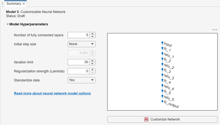
Display and Customize Network Architecture
After you create a customizable neural network model, the Summary tab displays the network architecture.
You can customize the network architecture by adding or removing layers, and editing layer properties. Click the Customize Network button to launch the Network Editor, a basic version of the Deep Network Designer (Deep Learning Toolbox) app that contains a subset of the layers listed in List of Deep Learning Layers (Deep Learning Toolbox). In the Network Editor, you cannot analyze a network for compression, or import a network from a file or the MATLAB workspace.
For a detailed example showing how to customize a neural network using the Network Editor, see Edit Customizable Neural Network Using Network Editor in Classification Learner or Regression Learner.
Analyze Network
You can display information about the layers in a customizable neural network by clicking Analyze Network in the Plots and Results section of the Learn tab. After you train the model, this option is also available in the Network Architecture section of the Summary tab.
To analyze your network while in the Network Editor, click Analyze in the Analysis section of the Designer tab. The app displays information about the layers, and checks the network for errors that prevent the model from being trained. Some common errors include size mismatches, missing connections, and missing layers. If your network contains errors, you can fix them using options in the Designer tab.
Set Hyperparameter Options
In the Model Hyperparameters section of the Summary tab, you can set these hyperparameters:
Number of fully connected layers — Specify the number of fully connected layers in the neural network, excluding the final fully connected layer for prediction. This option is not available after you make any changes to the network in the Network Editor. This option is also not available for the Residual Customizable Neural Network model preset.
Initial step size — Select one of these options:
Manual — Specify an initial step size to determine the initial Hessian approximation used in training the model. The default value is
0.001.Auto — The app determines the initial step size automatically.
None (default) — Do not use an initial step size.
Iteration limit — Specify the maximum number of training iterations.
Regularization strength (Lambda) — Specify the ridge (L2) regularization penalty term.
Standardize data — Specify whether to standardize the numeric predictors. If the predictors have widely different scales, standardizing can improve the fit. Standardizing the data is highly recommended. Note that because Regression Learner performs the data standardization, the Normalization value of a featureInputLayer block must be
"none"in a customizable neural network model.
For more information on these hyperparameters, see the fitrnet function page.
See Also
Topics
- Train Regression Models in Regression Learner App
- Edit Customizable Neural Network Using Network Editor in Classification Learner or Regression Learner
- Start a Classification Learner or Regression Learner Session
- Feature Selection and Feature Transformation Using Regression Learner App
- Visualize and Assess Model Performance in Regression Learner
- Export Regression Model to Predict New Data