fitrnet
Train neural network regression model
Syntax
Description
Use fitrnet to train a neural network for regression, such as
a feedforward, fully connected network. In a feedforward, fully connected network, the first
fully connected layer has a connection from the network input (predictor data), and each
subsequent layer has a connection from the previous layer. Each fully connected layer
multiplies the input by a weight matrix and then adds a bias vector. An activation function
follows each fully connected layer, excluding the last. The final fully connected layer
produces the network's output, namely predicted response values. For more information, see
Neural Network Structure.
Mdl = fitrnet(Tbl,ResponseVarName)Mdl trained using the
predictors in the table Tbl and the response values in the
ResponseVarName table variable.
You can use an array
ResponseVarName to specify multiple response variables. (since R2024b)
Mdl = fitrnet(Tbl,formula)Tbl. The input argument formula is an
explanatory model of the response and a subset of the predictor variables in
Tbl used to fit Mdl.
You can use formula to
specify multiple response variables. (since R2024b)
Mdl = fitrnet(___,Name=Value)LayerSizes and Activations name-value
arguments.
Cross-validation and hyperparameter optimization options are not supported for multiresponse regression.
[
also returns Mdl,AggregateOptimizationResults] = fitrnet(___)AggregateOptimizationResults, which contains
hyperparameter optimization results when you specify the
OptimizeHyperparameters and
HyperparameterOptimizationOptions name-value arguments. You must
also specify the ConstraintType and
ConstraintBounds options of
HyperparameterOptimizationOptions. You can use this syntax to
optimize on compact model size instead of cross-validation loss, and to perform a set of
multiple optimization problems that have the same options but different constraint
bounds.
Hyperparameter optimization options are not supported for multiresponse regression.
Examples
Train a neural network regression model, and assess the performance of the model on a test set.
Load the carbig data set, which contains measurements of cars made in the 1970s and early 1980s. Create a table containing the predictor variables Acceleration, Displacement, and so on, as well as the response variable MPG.
load carbig
cars = table(Acceleration,Displacement,Horsepower, ...
    Model_Year,Origin,Weight,MPG);
Remove rows of cars where the table has missing values.
cars = rmmissing(cars);
Categorize the cars based on whether they were made in the USA.
cars.Origin = categorical(cellstr(cars.Origin));
cars.Origin = mergecats(cars.Origin,["France","Japan",...
    "Germany","Sweden","Italy","England"],"NotUSA");
Partition the data into training and test sets. Use approximately 80% of the observations to train a neural network model, and 20% of the observations to test the performance of the trained model on new data. Use cvpartition to partition the data.
rng("default") % For reproducibility of the data partition
c = cvpartition(height(cars),"Holdout",0.20);
trainingIdx = training(c); % Training set indices
carsTrain = cars(trainingIdx,:);
testIdx = test(c); % Test set indices
carsTest = cars(testIdx,:);
Train a neural network regression model by passing the carsTrain training data to the fitrnet function. For better results, specify to standardize the predictor data.
Mdl = fitrnet(carsTrain,"MPG","Standardize",true)
Mdl =
  RegressionNeuralNetwork
           PredictorNames: {'Acceleration'  'Displacement'  'Horsepower'  'Model_Year'  'Origin'  'Weight'}
             ResponseName: 'MPG'
    CategoricalPredictors: 5
        ResponseTransform: 'none'
          NumObservations: 314
               LayerSizes: 10
              Activations: 'relu'
    OutputLayerActivation: 'none'
                   Solver: 'LBFGS'
          ConvergenceInfo: [1×1 struct]
          TrainingHistory: [708×7 table]


  Properties, Methods
Mdl is a trained RegressionNeuralNetwork model. You can use dot notation to access the properties of Mdl. For example, you can specify Mdl.TrainingHistory to get more information about the training history of the neural network model.
Evaluate the performance of the regression model on the test set by computing the test mean squared error (MSE). Smaller MSE values indicate better performance.
testMSE = loss(Mdl,carsTest,"MPG")testMSE = 7.1092
Configure the fully connected layers of the neural network.
Load the carbig data set, which contains measurements of cars made in the 1970s and early 1980s. Create a matrix X containing the predictor variables Acceleration, Cylinders, and so on. Store the response variable MPG in the variable Y.
load carbig
X = [Acceleration Cylinders Displacement Weight];
Y = MPG;
Delete rows of X and Y where either array has missing values.
R = rmmissing([X Y]);
X = R(:,1:end-1);
Y = R(:,end);
Partition the data into training data (XTrain and YTrain) and test data (XTest and YTest). Reserve approximately 20% of the observations for testing, and use the rest of the observations for training.
rng("default") % For reproducibility of the partition
c = cvpartition(length(Y),"Holdout",0.20);
trainingIdx = training(c); % Indices for the training set
XTrain = X(trainingIdx,:);
YTrain = Y(trainingIdx);
testIdx = test(c); % Indices for the test set
XTest = X(testIdx,:);
YTest = Y(testIdx);
Train a neural network regression model. Specify to standardize the predictor data, and to have 30 outputs in the first fully connected layer and 10 outputs in the second fully connected layer. By default, both layers use a rectified linear unit (ReLU) activation function. You can change the activation functions for the fully connected layers by using the Activations name-value argument.
Mdl = fitrnet(XTrain,YTrain,"Standardize",true, ...
    "LayerSizes",[30 10])
Mdl =
  RegressionNeuralNetwork
             ResponseName: 'Y'
    CategoricalPredictors: []
        ResponseTransform: 'none'
          NumObservations: 319
               LayerSizes: [30 10]
              Activations: 'relu'
    OutputLayerActivation: 'none'
                   Solver: 'LBFGS'
          ConvergenceInfo: [1×1 struct]
          TrainingHistory: [1000×7 table]


  Properties, Methods
Access the weights and biases for the fully connected layers of the trained model by using the LayerWeights and LayerBiases properties of Mdl. The first two elements of each property correspond to the values for the first two fully connected layers, and the third element corresponds to the values for the final fully connected layer for regression. For example, display the weights and biases for the first fully connected layer.
Mdl.LayerWeights{1}ans = 30×4
0.0123 0.0117 -0.0094 0.1175
-0.4081 -0.7849 -0.7201 -2.1720
0.6041 0.1680 -2.3952 0.0934
-3.2332 -2.8360 -1.8264 -1.5723
0.5851 1.5370 1.4623 0.6742
-0.2106 1.2830 -1.7489 -1.5556
0.4800 0.1012 -1.0044 -0.7959
1.8015 -0.5272 -0.7670 0.7496
-1.1428 -0.9902 0.2436 1.2288
-0.0833 -2.4265 0.8388 1.8597
0.1069 -0.6754 -2.4190 -2.1763
-0.4008 1.1705 2.0588 0.2282
0.6358 -0.4830 -1.6925 -1.1925
-0.9572 -1.2231 1.1647 1.0479
-0.5559 -0.0917 -3.6854 1.2579
⋮
Mdl.LayerBiases{1}ans = 30×1
-0.4450
-0.8751
-0.3872
-1.1345
0.4499
-2.1555
2.2111
1.2040
-1.4595
0.4639
-1.5912
-0.5617
0.6513
-2.0560
-2.2856
⋮
The final fully connected layer has one output. The number of layer outputs corresponds to the first dimension of the layer weights and layer biases.
size(Mdl.LayerWeights{end})ans = 1×2
1 10
size(Mdl.LayerBiases{end})ans = 1×2
1 1
To estimate the performance of the trained model, compute the test set mean squared error (MSE) for Mdl. Smaller MSE values indicate better performance.
testMSE = loss(Mdl,XTest,YTest)
testMSE =
18.3681
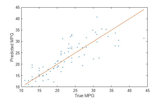
Compare the predicted test set response values to the true response values. Plot the predicted miles per gallon (MPG) along the vertical axis and the true MPG along the horizontal axis. Points on the reference line indicate correct predictions. A good model produces predictions that are scattered near the line.
testPredictions = predict(Mdl,XTest);
plot(YTest,testPredictions,".")
hold on
plot(YTest,YTest)
hold off
xlabel("True MPG")
ylabel("Predicted MPG")
Since R2025a
Specify a custom neural network architecture using Deep Learning Toolbox™.
To specify a neural network of fully connected layers connected in series, use arguments like the LayerSizes argument to configure the neural network architecture. For neural networks with more complex architecture (such as, neural networks with skip connections), you can specify the architecture using the Network name-value argument with a dlnetwork object.
Load the carbig data set.
load carbig
X = [Acceleration Cylinders Displacement Weight];
Y = MPG;
Delete rows of the data where either array has missing values.
R = rmmissing([X Y]);
X = R(:,1:end-1);
Y = R(:,end);
Partition the data into training data (XTrain and YTrain) and test data (XTest and YTest). Reserve approximately 20% of the observations for testing, and use the rest of the observations for training.
rng("default") % For reproducibility of the partition
c = cvpartition(length(Y),Holdout=0.2);
trainingIdx = training(c); % Indices for the training set
XTrain = X(trainingIdx,:);
YTrain = Y(trainingIdx);
testIdx = test(c); % Indices for the test set
XTest = X(testIdx,:);
YTest = Y(testIdx);
Define a neural network architecture with these characteristics:
A feature input layer with an input size that matches the number of predictors.
Three fully connected layers followed by ReLU layers, connected in series, where the fully connected layers have output sizes of 12, and addition layers after the second and third fully connected layers.
Skip connections around the second and third fully connected layers using the addition layers.
A final fully connected layer with an output size that matches the number of responses.
inputSize = size(XTrain,2);
outputSize = size(YTrain,2);

net = dlnetwork;

layers = [
    featureInputLayer(inputSize)
    fullyConnectedLayer(12)
    reluLayer(Name="relu1")

    fullyConnectedLayer(12)

    additionLayer(2,Name="add2")
    reluLayer(Name="relu2")

    fullyConnectedLayer(12)
    additionLayer(2,Name="add3")
    reluLayer

    fullyConnectedLayer(outputSize)];

net = addLayers(net,layers);
net = connectLayers(net,"relu1","add2/in2");
net = connectLayers(net,"relu2","add3/in2");
Visualize the neural network architecture in a plot.
figure
plot(net)

Train a neural network regression model.
Mdl = fitrnet(XTrain,YTrain,Network=net,Standardize=true)
Mdl =
  RegressionNeuralNetwork
             ResponseName: 'Y'
    CategoricalPredictors: []
        ResponseTransform: 'none'
          NumObservations: 319
               LayerSizes: []
              Activations: ''
    OutputLayerActivation: ''
                   Solver: 'LBFGS'
          ConvergenceInfo: [1×1 struct]
          TrainingHistory: [1000×7 table]

  View network information using dlnetwork.


  Properties, Methods
Evaluate the performance of the regression model on the test set by computing the test mean squared error (MSE). Smaller values indicate better predictive accuracy.
testMSE = loss(Mdl,XTest,YTest)
testMSE =
14.3926
At each iteration of the training process, compute the validation loss of the neural network. Stop the training process early if the validation loss reaches a reasonable minimum.
Load the patients data set. Create a table from the data set. Each row corresponds to one patient, and each column corresponds to a diagnostic variable. Use the Systolic variable as the response variable, and the rest of the variables as predictors.
load patients
tbl = table(Age,Diastolic,Gender,Height,Smoker,Weight,Systolic);
Separate the data into a training set tblTrain and a validation set tblValidation. The software reserves approximately 30% of the observations for the validation data set and uses the rest of the observations for the training data set.
rng("default") % For reproducibility of the partition
c = cvpartition(size(tbl,1),"Holdout",0.30);
trainingIndices = training(c);
validationIndices = test(c);
tblTrain = tbl(trainingIndices,:);
tblValidation = tbl(validationIndices,:);
Train a neural network regression model by using the training set. Specify the Systolic column of tblTrain as the response variable. Evaluate the model at each iteration by using the validation set. Specify to display the training information at each iteration by using the Verbose name-value argument. By default, the training process ends early if the validation loss is greater than or equal to the minimum validation loss computed so far, six times in a row. To change the number of times the validation loss is allowed to be greater than or equal to the minimum, specify the ValidationPatience name-value argument.
Mdl = fitrnet(tblTrain,"Systolic", ...
    "ValidationData",tblValidation, ...
    "Verbose",1);
|==========================================================================================|
| Iteration  | Train Loss | Gradient   | Step       | Iteration  | Validation | Validation |
|            |            |            |            | Time (sec) | Loss       | Checks     |
|==========================================================================================|
|           1|  516.021993| 3220.880047|    0.644473|    0.007097|  568.289202|           0|
|           2|  313.056754|  229.931405|    0.067026|    0.004018|  304.023695|           0|
|           3|  308.461807|  277.166516|    0.011122|    0.001095|  296.935608|           0|
|           4|  262.492770|  844.627934|    0.143022|    0.000190|  240.559640|           0|
|           5|  169.558740| 1131.714363|    0.336463|    0.000156|  152.531663|           0|
|           6|   89.134368|  362.084104|    0.382677|    0.000298|   83.147478|           0|
|           7|   83.309729|  994.830303|    0.199923|    0.000120|   76.634122|           0|
|           8|   70.731524|  327.637362|    0.041366|    0.000114|   66.421750|           0|
|           9|   66.650091|  124.369963|    0.125232|    0.000108|   65.914063|           0|
|          10|   66.404753|   36.699328|    0.016768|    0.000108|   65.357335|           0|
|==========================================================================================|
| Iteration  | Train Loss | Gradient   | Step       | Iteration  | Validation | Validation |
|            |            |            |            | Time (sec) | Loss       | Checks     |
|==========================================================================================|
|          11|   66.357143|   46.712988|    0.009405|    0.000771|   65.306106|           0|
|          12|   66.268225|   54.079264|    0.007953|    0.000709|   65.234391|           0|
|          13|   65.788550|   99.453225|    0.030942|    0.000169|   64.869708|           0|
|          14|   64.821095|  186.344649|    0.048078|    0.000124|   64.191533|           0|
|          15|   62.353896|  319.273873|    0.107160|    0.000113|   62.618374|           0|
|          16|   57.836593|  447.826470|    0.184985|    0.000114|   60.087065|           0|
|          17|   51.188884|  524.631067|    0.253062|    0.000113|   56.646294|           0|
|          18|   41.755601|  189.072516|    0.318515|    0.000110|   49.046823|           0|
|          19|   37.539854|   78.602559|    0.382284|    0.000106|   44.633562|           0|
|          20|   36.845322|  151.837884|    0.211286|    0.000111|   47.291367|           1|
|==========================================================================================|
| Iteration  | Train Loss | Gradient   | Step       | Iteration  | Validation | Validation |
|            |            |            |            | Time (sec) | Loss       | Checks     |
|==========================================================================================|
|          21|   36.218289|   62.826818|    0.142748|    0.000111|   46.139104|           2|
|          22|   35.776921|   53.606315|    0.215188|    0.000128|   46.170460|           3|
|          23|   35.729085|   24.400342|    0.060096|    0.000434|   45.318023|           4|
|          24|   35.622031|    9.602277|    0.121153|    0.000112|   45.791861|           5|
|          25|   35.573317|   10.735070|    0.126854|    0.000105|   46.062826|           6|
|==========================================================================================|
Create a plot that compares the training mean squared error (MSE) and the validation MSE at each iteration. By default, fitrnet stores the loss information inside the TrainingHistory property of the object Mdl. You can access this information by using dot notation.
iteration = Mdl.TrainingHistory.Iteration;
trainLosses = Mdl.TrainingHistory.TrainingLoss;
valLosses = Mdl.TrainingHistory.ValidationLoss;
plot(iteration,trainLosses,iteration,valLosses)
legend(["Training","Validation"])
xlabel("Iteration")
ylabel("Mean Squared Error")

Check the iteration that corresponds to the minimum validation MSE. The final returned model Mdl is the model trained at this iteration.
[~,minIdx] = min(valLosses);
iteration(minIdx)
ans =
19
Assess the cross-validation loss of neural network models with different regularization strengths, and choose the regularization strength corresponding to the best performing model.
Load the carbig data set, which contains measurements of cars made in the 1970s and early 1980s. Create a table containing the predictor variables Acceleration, Displacement, and so on, as well as the response variable MPG.
load carbig
cars = table(Acceleration,Displacement,Horsepower, ...
    Model_Year,Origin,Weight,MPG);
Delete rows of cars where the table has missing values.
cars = rmmissing(cars);
Categorize the cars based on whether they were made in the USA.
cars.Origin = categorical(cellstr(cars.Origin));
cars.Origin = mergecats(cars.Origin,["France","Japan", ...
    "Germany","Sweden","Italy","England"],"NotUSA");
Create a cvpartition object for 5-fold cross-validation. cvp partitions the data into five folds, where each fold has roughly the same number of observations. Set the random seed to the default value for reproducibility of the partition.
rng("default")
n = size(cars,1);
cvp = cvpartition(n,"KFold",5);
Compute the cross-validation mean squared error (MSE) for neural network regression models with different regularization strengths. Try regularization strengths on the order of 1/n, where n is the number of observations. Specify to standardize the data before training the neural network models.
1/n
ans = 0.0026
lambda = (0:0.5:5)*1e-3;
cvloss = zeros(length(lambda),1);
for i = 1:length(lambda)
    cvMdl = fitrnet(cars,"MPG","Lambda",lambda(i), ...
        "CVPartition",cvp,"Standardize",true);
    cvloss(i) = kfoldLoss(cvMdl);
end
Plot the results. Find the regularization strength corresponding to the lowest cross-validation MSE.
plot(lambda,cvloss)
xlabel("Regularization Strength")
ylabel("Cross-Validation Loss")

[~,idx] = min(cvloss);
bestLambda = lambda(idx)
bestLambda = 0.0045
Train a neural network regression model using the bestLambda regularization strength.
Mdl = fitrnet(cars,"MPG","Lambda",bestLambda, ...
    "Standardize",true)
Mdl =
  RegressionNeuralNetwork
           PredictorNames: {'Acceleration'  'Displacement'  'Horsepower'  'Model_Year'  'Origin'  'Weight'}
             ResponseName: 'MPG'
    CategoricalPredictors: 5
        ResponseTransform: 'none'
          NumObservations: 392
               LayerSizes: 10
              Activations: 'relu'
    OutputLayerActivation: 'none'
                   Solver: 'LBFGS'
          ConvergenceInfo: [1×1 struct]
          TrainingHistory: [761×7 table]


  Properties, Methods
Create a neural network with low error by using the OptimizeHyperparameters argument. This argument causes fitrnet to minimize cross-validation loss over some problem hyperparameters by using Bayesian optimization.
Load the carbig data set, which contains measurements of cars made in the 1970s and early 1980s. Create a table containing the predictor variables Acceleration, Displacement, and so on, as well as the response variable MPG.
load carbig
cars = table(Acceleration,Displacement,Horsepower, ...
    Model_Year,Origin,Weight,MPG);
Delete rows of cars where the table has missing values.
cars = rmmissing(cars);
Categorize the cars based on whether they were made in the USA.
cars.Origin = categorical(cellstr(cars.Origin));
cars.Origin = mergecats(cars.Origin,["France","Japan",...
    "Germany","Sweden","Italy","England"],"NotUSA");
Partition the data into training and test sets. Use approximately 80% of the observations to train a neural network model, and 20% of the observations to test the performance of the trained model on new data. Use cvpartition to partition the data.
rng("default") % For reproducibility of the data partition
c = cvpartition(height(cars),Holdout=0.20);

trainingIdx = training(c);
carsTrain = cars(trainingIdx,:);

testIdx = test(c);
carsTest = cars(testIdx,:);
Train a regression neural network using the OptimizeHyperparameters argument set to "auto". For reproducibility, set the AcquisitionFunctionName to "expected-improvement-plus" in a HyperparameterOptimizationOptions object. fitrnet performs Bayesian optimization by default. To use grid search or random search, set the Optimizer value in HyperparameterOptimizationOptions.
rng("default") % For reproducibility
hpoOptions = hyperparameterOptimizationOptions(AcquisitionFunctionName="expected-improvement-plus");
Mdl = fitrnet(carsTrain,"MPG",OptimizeHyperparameters="auto", ...
    HyperparameterOptimizationOptions=hpoOptions)
|============================================================================================================================================|
| Iter | Eval   | Objective:  | Objective   | BestSoFar   | BestSoFar   |  Activations |  Standardize |       Lambda |            LayerSizes |
|      | result | log(1+loss) | runtime     | (observed)  | (estim.)    |              |              |              |                       |
|============================================================================================================================================|
|    1 | Best   |       2.224 |      8.8873 |       2.224 |       2.224 |         relu |         true |        3.841 | [101  47  15]         |
|    2 | Accept |      3.2826 |      6.1492 |       2.224 |      2.2661 |      sigmoid |        false |   7.5401e-07 | [100  17]             |
|    3 | Best   |      2.0931 |      2.0117 |      2.0931 |      2.1105 |         relu |         true |      0.01569 |  15                   |
|    4 | Accept |      2.5142 |      3.2311 |      2.0931 |      2.1166 |         none |         true |   0.00016461 | [  2 145   8]         |
|    5 | Accept |      3.0244 |     0.39902 |      2.0931 |      2.0932 |         relu |         true |    3.566e-08 |  1                    |
|    6 | Accept |      2.8085 |      2.4867 |      2.0931 |      2.1508 |         relu |         true |      0.10807 | [ 72   1]             |
|    7 | Accept |      2.1352 |      2.1477 |      2.0931 |      2.0936 |         relu |         true |    0.0093614 |  17                   |
|    8 | Accept |      2.3367 |      0.8332 |      2.0931 |      2.0935 |         relu |         true |       2.1553 |  57                   |
|    9 | Accept |      2.3387 |     0.53068 |      2.0931 |      2.0935 |         relu |         true |        9.321 | [  4  70  17]         |
|   10 | Best   |        2.08 |      3.0651 |        2.08 |        2.08 |         relu |         true |      0.28308 | [ 30  10   8]         |
|   11 | Accept |      2.6096 |      2.2261 |        2.08 |      2.0801 |         relu |         true |    0.0025126 | [ 11   4   3]         |
|   12 | Accept |      2.2917 |      0.4798 |        2.08 |      2.0894 |         relu |         true |     0.076717 |  2                    |
|   13 | Accept |      2.6177 |      2.5626 |        2.08 |        2.08 |         relu |         true |   0.00090431 |  57                   |
|   14 | Accept |      2.0991 |      11.377 |        2.08 |      2.0801 |         relu |         true |      0.60466 | [ 18  91 148]         |
|   15 | Accept |      6.3855 |     0.17813 |        2.08 |      2.0799 |         relu |         true |       92.264 |  276                  |
|   16 | Accept |      2.5619 |      2.1814 |        2.08 |        2.08 |         relu |         true |        11.32 | [ 49 291]             |
|   17 | Accept |      6.3901 |     0.19635 |        2.08 |      2.0811 |         relu |         true |       104.94 | [ 58  30 164]         |
|   18 | Accept |      2.5141 |      1.6898 |        2.08 |       2.081 |         none |         true |    0.0034524 | [  8 109]             |
|   19 | Accept |      3.5535 |      5.8988 |        2.08 |      2.0809 |         relu |         true |   2.6214e-05 | [229   7   1]         |
|   20 | Accept |      2.5151 |     0.14441 |        2.08 |      2.0809 |         relu |         true |      0.32515 |  1                    |
|============================================================================================================================================|
| Iter | Eval   | Objective:  | Objective   | BestSoFar   | BestSoFar   |  Activations |  Standardize |       Lambda |            LayerSizes |
|      | result | log(1+loss) | runtime     | (observed)  | (estim.)    |              |              |              |                       |
|============================================================================================================================================|
|   21 | Accept |      2.2322 |      3.2178 |        2.08 |      2.0809 |         relu |         true |     0.016195 | [  1 187]             |
|   22 | Accept |      2.0928 |      7.6525 |        2.08 |      2.1618 |         relu |         true |      0.47387 | [230  12]             |
|   23 | Accept |      2.5142 |       6.604 |        2.08 |      2.1619 |         none |         true |   1.0862e-05 | [122  27]             |
|   24 | Accept |      2.5136 |     0.33308 |        2.08 |      2.0811 |         none |         true |     0.049625 |  23                   |
|   25 | Accept |      2.5142 |      1.8753 |        2.08 |       2.081 |         none |         true |   1.2062e-06 | [  1 143]             |
|   26 | Accept |      2.5142 |      0.1864 |        2.08 |      2.1637 |         none |         true |   1.6616e-07 |  236                  |
|   27 | Accept |      2.5147 |     0.41565 |        2.08 |      2.1636 |         none |         true |      0.79119 | [  4  94]             |
|   28 | Accept |      2.6721 |     0.29712 |        2.08 |      2.1635 |         none |         true |       12.606 | [196   4  45]         |
|   29 | Accept |      6.4126 |    0.091009 |        2.08 |      2.1697 |         none |         true |       314.02 |  3                    |
|   30 | Accept |      2.5242 |      11.762 |        2.08 |      2.1672 |         tanh |         true |     0.040731 | [ 20  20 286]         |

__________________________________________________________
Optimization completed.
MaxObjectiveEvaluations of 30 reached.
Total function evaluations: 30
Total elapsed time: 101.0126 seconds
Total objective function evaluation time: 89.1111

Best observed feasible point:
    Activations    Standardize    Lambda       LayerSizes
    ___________    ___________    _______    ______________

       relu           true        0.28308    30    10     8

Observed objective function value = 2.08
Estimated objective function value = 2.3123
Function evaluation time = 3.0651

Best estimated feasible point (according to models):
    Activations    Standardize    Lambda     LayerSizes
    ___________    ___________    _______    __________

       relu           true        0.47387    230     12

Estimated objective function value = 2.1672
Estimated function evaluation time = 7.6538

Mdl =
  RegressionNeuralNetwork
                       PredictorNames: {'Acceleration'  'Displacement'  'Horsepower'  'Model_Year'  'Origin'  'Weight'}
                         ResponseName: 'MPG'
                CategoricalPredictors: 5
                    ResponseTransform: 'none'
                      NumObservations: 314
    HyperparameterOptimizationResults: [1×1 classreg.learning.paramoptim.SupervisedLearningBayesianOptimization]
                           LayerSizes: [230 12]
                          Activations: 'relu'
                OutputLayerActivation: 'none'
                               Solver: 'LBFGS'
                      ConvergenceInfo: [1×1 struct]
                      TrainingHistory: [1000×7 table]


  Properties, Methods
The trained model Mdl corresponds to the best estimated feasible point and uses the same hyperparameter values for Activations, Standardize, Lambda, and LayerSizes.
Find the hyperparameter values used to train Mdl by using the bestPoint function. By default, bestPoint uses the same best point criterion used by fitrnet during the hyperparameter optimization ("min-visited-upper-confidence-interval"). In general, fit functions determine the best hyperparameter values based on the "min-visited-upper-confidence-interval" criterion (instead of the "min-observed" criterion) to avoid overfitting to noise in the data set.
bestEstimatedPoint = bestPoint(Mdl.HyperparameterOptimizationResults)
bestEstimatedPoint=1×7 table
    NumLayers    Activations    Standardize    Lambda     Layer_1_Size    Layer_2_Size    Layer_3_Size
    _________    ___________    ___________    _______    ____________    ____________    ____________

        2           relu           true        0.47387        230              12             NaN
Verify that the results match the properties of Mdl. Note that the Mu and Sigma properties of a RegressionNeuralNetwork object are nonempty when the neural network model uses standardization.
modelProperties = table(length(Mdl.LayerSizes), ...
    string(Mdl.Activations), ...
    struct(Means=Mdl.Mu,StandardDeviations=Mdl.Sigma), ...
    Mdl.ModelParameters.Lambda,Mdl.LayerSizes, ...
    VariableNames=["NumLayers","Activations","Standardize", ...
    "Lambda","LayerSizes"])
modelProperties=1×5 table
    NumLayers    Activations    Standardize    Lambda     LayerSizes
    _________    ___________    ___________    _______    __________

        2          "relu"       1×1 struct     0.47387    230     12
modelProperties.Standardize
ans = struct with fields:
                 Means: [15.5825 192.8041 103.8344 75.9968 0 0 2.9605e+03]
    StandardDeviations: [2.8095 104.4709 38.8078 3.6940 1 1 843.5999]
Find the mean squared error of the optimized model on the test data set.
testMSE = loss(Mdl,carsTest,"MPG")testMSE = 7.2269
Create a neural network with low error by using the OptimizeHyperparameters argument. This argument causes fitrnet to search for hyperparameters that give a model with low cross-validation error. Use the hyperparameters function to specify larger-than-default values for the number of layers used and the layer size range.
Load the carbig data set, which contains measurements of cars made in the 1970s and early 1980s. Create a table containing the predictor variables Acceleration, Displacement, and so on, as well as the response variable MPG.
load carbig
cars = table(Acceleration,Displacement,Horsepower, ...
    Model_Year,Origin,Weight,MPG);
Delete rows of cars where the table has missing values.
cars = rmmissing(cars);
Categorize the cars based on whether they were made in the USA.
cars.Origin = categorical(cellstr(cars.Origin));
cars.Origin = mergecats(cars.Origin,["France","Japan",...
    "Germany","Sweden","Italy","England"],"NotUSA");
Partition the data into training and test sets. Use approximately 80% of the observations to train a neural network model, and 20% of the observations to test the performance of the trained model on new data. Use cvpartition to partition the data.
rng("default") % For reproducibility of the data partition
c = cvpartition(height(cars),"Holdout",0.20);
trainingIdx = training(c); % Training set indices
carsTrain = cars(trainingIdx,:);
testIdx = test(c); % Test set indices
carsTest = cars(testIdx,:);
List the hyperparameters available for this problem of fitting the MPG response.
params = hyperparameters("fitrnet",carsTrain,"MPG");
for ii = 1:length(params)
    disp(ii);disp(params(ii))
end
     1

  optimizableVariable with properties:

         Name: 'NumLayers'
        Range: [1 3]
         Type: 'integer'
    Transform: 'none'
     Optimize: 1

     2

  optimizableVariable with properties:

         Name: 'Activations'
        Range: {'relu'  'tanh'  'sigmoid'  'none'}
         Type: 'categorical'
    Transform: 'none'
     Optimize: 1

     3

  optimizableVariable with properties:

         Name: 'Standardize'
        Range: {'true'  'false'}
         Type: 'categorical'
    Transform: 'none'
     Optimize: 1

     4

  optimizableVariable with properties:

         Name: 'Lambda'
        Range: [3.1847e-08 318.4713]
         Type: 'real'
    Transform: 'log'
     Optimize: 1

     5

  optimizableVariable with properties:

         Name: 'LayerWeightsInitializer'
        Range: {'glorot'  'he'}
         Type: 'categorical'
    Transform: 'none'
     Optimize: 0

     6

  optimizableVariable with properties:

         Name: 'LayerBiasesInitializer'
        Range: {'zeros'  'ones'}
         Type: 'categorical'
    Transform: 'none'
     Optimize: 0

     7

  optimizableVariable with properties:

         Name: 'Layer_1_Size'
        Range: [1 300]
         Type: 'integer'
    Transform: 'log'
     Optimize: 1

     8

  optimizableVariable with properties:

         Name: 'Layer_2_Size'
        Range: [1 300]
         Type: 'integer'
    Transform: 'log'
     Optimize: 1

     9

  optimizableVariable with properties:

         Name: 'Layer_3_Size'
        Range: [1 300]
         Type: 'integer'
    Transform: 'log'
     Optimize: 1

    10

  optimizableVariable with properties:

         Name: 'Layer_4_Size'
        Range: [1 300]
         Type: 'integer'
    Transform: 'log'
     Optimize: 0

    11

  optimizableVariable with properties:

         Name: 'Layer_5_Size'
        Range: [1 300]
         Type: 'integer'
    Transform: 'log'
     Optimize: 0
To try more layers than the default of 1 through 3, set the range of NumLayers (optimizable variable 1) to its maximum allowable size, [1 5]. Also, set Layer_4_Size and Layer_5_Size (optimizable variables 10 and 11, respectively) to be optimized.
params(1).Range = [1 5];
params(10).Optimize = true;
params(11).Optimize = true;
Set the range of all layer sizes (optimizable variables 7 through 11) to [1 400] instead of the default [1 300].
for ii = 7:11
    params(ii).Range = [1 400];
end
Train a regression neural network using the OptimizeHyperparameters argument set to params. For reproducibility, set the AcquisitionFunctionName to "expected-improvement-plus" in a HyperparameterOptimizationOptions structure. To attempt to get a better solution, set the number of optimization steps to 60 instead of the default 30.
rng("default") % For reproducibility
Mdl = fitrnet(carsTrain,"MPG","OptimizeHyperparameters",params, ...
    "HyperparameterOptimizationOptions", ...
    struct("AcquisitionFunctionName","expected-improvement-plus", ...
    "MaxObjectiveEvaluations",60))
|============================================================================================================================================|
| Iter | Eval   | Objective:  | Objective   | BestSoFar   | BestSoFar   |  Activations |  Standardize |       Lambda |            LayerSizes |
|      | result | log(1+loss) | runtime     | (observed)  | (estim.)    |              |              |              |                       |
|============================================================================================================================================|
|    1 | Best   |      4.9294 |      2.2802 |      4.9294 |      4.9294 |      sigmoid |        false |       70.242 | [  3  22 223]         |
|    2 | Best   |      2.2094 |      4.6982 |      2.2094 |      2.3176 |         relu |         true |     0.089397 | [  2  95]             |
|    3 | Accept |      2.9188 |      26.816 |      2.2094 |      2.2959 |      sigmoid |        false |   2.5899e-07 | [303  60  59]         |
|    4 | Accept |      3.5207 |      3.7559 |      2.2094 |      2.2898 |         relu |        false |   5.1748e-05 | [102   5  15   1]     |
|    5 | Accept |      2.2303 |      3.0885 |      2.2094 |      2.2156 |         relu |         true |     0.095678 | [  2  68]             |
|    6 | Accept |      2.2876 |      2.5587 |      2.2094 |      2.2148 |         relu |         true |    0.0012079 | [  2  72]             |
|    7 | Accept |      6.3902 |     0.11084 |      2.2094 |       2.221 |         relu |         true |       105.14 | [  2  22   3]         |
|    8 | Accept |      2.3386 |     0.31716 |      2.2094 |      2.2483 |         relu |         true |        5.677 | [  3  74]             |
|    9 | Accept |      4.5658 |     0.39478 |      2.2094 |      2.2197 |      sigmoid |        false |       15.788 | [  5  17  58]         |
|   10 | Accept |      3.5436 |      19.201 |      2.2094 |      2.2189 |         relu |        false |   0.00024703 | [  2 269 182 100]     |
|   11 | Accept |      6.3893 |      0.1489 |      2.2094 |       2.221 |         relu |         true |       102.48 | [  1 121]             |
|   12 | Accept |      6.3682 |     0.17312 |      2.2094 |      2.2117 |         relu |         true |       63.216 | [  4 228]             |
|   13 | Best   |      2.1148 |      8.9104 |      2.1148 |      2.1147 |         relu |         true |       1.5399 | [ 41  55  31]         |
|   14 | Accept |      3.0744 |      4.6834 |      2.1148 |      2.1147 |         relu |         true |    0.0095522 | [ 61  27   4]         |
|   15 | Accept |      2.1437 |       2.059 |      2.1148 |      2.1136 |         relu |         true |       1.3153 | [  3 104  12  12  10] |
|   16 | Accept |      3.7846 |      4.6642 |      2.1148 |      2.1139 |         relu |         true |    0.0002198 | [ 19  36 210   1]     |
|   17 | Accept |      4.1318 |      0.2961 |      2.1148 |      2.1139 |      sigmoid |        false |   3.5617e-06 | [  6  83 171  81]     |
|   18 | Accept |      4.1318 |      0.1118 |      2.1148 |       2.114 |      sigmoid |        false |   3.2115e-08 |  1                    |
|   19 | Accept |      2.2453 |      3.4234 |      2.1148 |      2.1181 |         relu |         true |       2.9626 | [158   6]             |
|   20 | Accept |      2.2009 |      1.5857 |      2.1148 |      2.1185 |         relu |         true |    0.0022809 |  7                    |
|============================================================================================================================================|
| Iter | Eval   | Objective:  | Objective   | BestSoFar   | BestSoFar   |  Activations |  Standardize |       Lambda |            LayerSizes |
|      | result | log(1+loss) | runtime     | (observed)  | (estim.)    |              |              |              |                       |
|============================================================================================================================================|
|   21 | Accept |       7.132 |      5.5647 |      2.1148 |      2.1199 |         relu |        false |   8.6736e-07 | [ 41  13  72  85   7] |
|   22 | Accept |      10.394 |      0.3686 |      2.1148 |      2.1241 |         relu |        false |     0.017821 | [211   6]             |
|   23 | Accept |      2.5956 |      6.3171 |      2.1148 |      2.1238 |      sigmoid |        false |      0.07769 |  197                  |
|   24 | Accept |      2.6608 |      10.798 |      2.1148 |      2.1239 |      sigmoid |        false |    0.0082243 | [  4   8 262]         |
|   25 | Accept |      2.9195 |      5.2284 |      2.1148 |      2.1239 |      sigmoid |        false |    0.0005668 | [ 12  15   1   2]     |
|   26 | Accept |      4.1306 |      12.313 |      2.1148 |      2.1238 |      sigmoid |        false |      0.54341 | [ 20 182   3 148]     |
|   27 | Best   |      2.0816 |      14.261 |      2.0816 |      2.0818 |         tanh |         true |      0.05702 | [  2  37 260]         |
|   28 | Accept |      2.3947 |      36.852 |      2.0816 |      2.0818 |         tanh |         true |    0.0097787 | [ 85 321 120]         |
|   29 | Accept |      3.6249 |      11.042 |      2.0816 |      2.0819 |         tanh |         true |       0.5126 | [  7 390   1]         |
|   30 | Accept |      2.2016 |       5.135 |      2.0816 |      2.0819 |         tanh |         true |   0.00037508 | [  2   6   1  11  38] |
|   31 | Accept |      2.9537 |       26.04 |      2.0816 |      2.0819 |         tanh |         true |   4.5464e-05 | [  6 313  97]         |
|   32 | Accept |      3.1535 |      26.879 |      2.0816 |      2.0818 |         tanh |         true |    0.0014277 | [ 40  31   1 269 106] |
|   33 | Accept |      3.3028 |      15.409 |      2.0816 |      2.0821 |         tanh |         true |     0.027527 | [ 17  23   6  36 194] |
|   34 | Accept |      2.2361 |      9.6391 |      2.0816 |      2.0822 |         tanh |         true |   0.00029403 | [  2 371]             |
|   35 | Accept |      2.3367 |      45.086 |      2.0816 |      2.0824 |         relu |         true |    0.0020365 | [  4   3   1 237 396] |
|   36 | Accept |        3.12 |      15.853 |      2.0816 |      2.0823 |         tanh |         true |   0.00014636 | [ 60   3   7  17 230] |
|   37 | Accept |      2.7592 |      13.405 |      2.0816 |      2.0823 |         tanh |         true |   2.4356e-06 | [286   3  17]         |
|   38 | Accept |       2.788 |      5.4946 |      2.0816 |      2.0822 |         tanh |         true |    1.291e-07 | [  8  24  59]         |
|   39 | Best   |      2.0702 |      11.628 |      2.0702 |      2.0704 |         relu |         true |      0.54965 | [198   8 201   3]     |
|   40 | Accept |      3.5354 |      3.3932 |      2.0702 |      2.0705 |         relu |         true |      0.16523 | [  1  27   7   2 362] |
|============================================================================================================================================|
| Iter | Eval   | Objective:  | Objective   | BestSoFar   | BestSoFar   |  Activations |  Standardize |       Lambda |            LayerSizes |
|      | result | log(1+loss) | runtime     | (observed)  | (estim.)    |              |              |              |                       |
|============================================================================================================================================|
|   41 | Accept |      4.1318 |     0.79934 |      2.0702 |      2.0704 |      sigmoid |        false |     0.033173 | [ 29  53 144   1 385] |
|   42 | Accept |      2.8183 |      26.331 |      2.0702 |      2.0704 |         tanh |         true |   5.7724e-07 | [ 96  19 126  21 394] |
|   43 | Accept |      2.4177 |        3.66 |      2.0702 |      2.0704 |      sigmoid |         true |    0.0021392 | [  8  54]             |
|   44 | Accept |      2.2465 |      3.3487 |      2.0702 |      2.0704 |      sigmoid |         true |   0.00023471 | [  1   2   4   3]     |
|   45 | Accept |      3.1464 |       17.29 |      2.0702 |      2.0704 |      sigmoid |         true |   0.00063794 | [117  29 121   1 361] |
|   46 | Accept |       2.487 |      7.8231 |      2.0702 |      2.0704 |      sigmoid |         true |   2.4032e-05 | [  5   2 261]         |
|   47 | Accept |      2.0921 |      7.7871 |      2.0702 |      2.0704 |      sigmoid |         true |     0.030571 | [ 19   5 217]         |
|   48 | Accept |      2.3277 |     0.82029 |      2.0702 |      2.0704 |      sigmoid |         true |      0.23642 | [ 24  51]             |
|   49 | Accept |      4.1318 |     0.71976 |      2.0702 |      2.0704 |      sigmoid |         true |     0.065489 | [  8   6 100   7 215] |
|   50 | Accept |      4.1387 |     0.55016 |      2.0702 |      2.0704 |      sigmoid |         true |       3.3184 | [  9 127 114]         |
|   51 | Accept |      2.7828 |      19.959 |      2.0702 |      2.0704 |      sigmoid |         true |   4.8063e-05 | [388  15   2   3 177] |
|   52 | Accept |      3.9381 |      5.0077 |      2.0702 |      2.0704 |      sigmoid |         true |   1.1708e-06 | [  5 113  39 244  11] |
|   53 | Accept |      2.2112 |      7.9564 |      2.0702 |      2.0704 |      sigmoid |         true |     0.010242 | [ 90  26  11]         |
|   54 | Accept |      2.5142 |      1.0549 |      2.0702 |      2.0704 |         none |         true |    0.0010158 | [  2   2]             |
|   55 | Accept |      2.5141 |      1.6621 |      2.0702 |      2.0704 |         none |         true |      0.01172 | [  6   4  24  46]     |
|   56 | Accept |      2.5141 |      26.813 |      2.0702 |      2.0704 |         none |         true |     0.007888 | [ 67 252  34  90 388] |
|   57 | Accept |      2.5143 |      24.783 |      2.0702 |      2.0704 |         none |         true |   0.00011512 | [123   3   7 148 346] |
|   58 | Accept |      2.5142 |      1.1118 |      2.0702 |      2.0704 |         none |         true |   1.8517e-05 | [  5   5]             |
|   59 | Accept |      2.5142 |      5.6736 |      2.0702 |      2.0705 |         none |         true |   3.5558e-06 | [ 65  12  63  20 372] |
|   60 | Accept |      2.5142 |     0.35545 |      2.0702 |      2.0705 |         none |         true |   5.0732e-07 | [  4   6  17 246]     |

__________________________________________________________
Optimization completed.
MaxObjectiveEvaluations of 60 reached.
Total function evaluations: 60
Total elapsed time: 563.2365 seconds
Total objective function evaluation time: 533.49

Best observed feasible point:
    Activations    Standardize    Lambda            LayerSizes
    ___________    ___________    _______    ________________________

       relu           true        0.54965    198      8    201      3

Observed objective function value = 2.0702
Estimated objective function value = 2.0705
Function evaluation time = 11.6275

Best estimated feasible point (according to models):
    Activations    Standardize    Lambda            LayerSizes
    ___________    ___________    _______    ________________________

       relu           true        0.54965    198      8    201      3

Estimated objective function value = 2.0705
Estimated function evaluation time = 10.9307

Mdl =
  RegressionNeuralNetwork
                       PredictorNames: {'Acceleration'  'Displacement'  'Horsepower'  'Model_Year'  'Origin'  'Weight'}
                         ResponseName: 'MPG'
                CategoricalPredictors: 5
                    ResponseTransform: 'none'
                      NumObservations: 314
    HyperparameterOptimizationResults: [1×1 classreg.learning.paramoptim.SupervisedLearningBayesianOptimization]
                           LayerSizes: [198 8 201 3]
                          Activations: 'relu'
                OutputLayerActivation: 'none'
                               Solver: 'LBFGS'
                      ConvergenceInfo: [1×1 struct]
                      TrainingHistory: [1000×7 table]


  Properties, Methods
Find the mean squared error of the resulting model on the test data set.
testMSE = loss(Mdl,carsTest,"MPG")testMSE = 7.0574
Since R2024b
Create a regression neural network with more than one response variable.
Load the carbig data set, which contains measurements of cars made in the 1970s and early 1980s. Create a table containing the predictor variables Displacement, Horsepower, and so on, as well as the response variables Acceleration and MPG. Display the first eight rows of the table.
load carbig
cars = table(Displacement,Horsepower,Model_Year, ...
    Origin,Weight,Acceleration,MPG);
head(cars)
    Displacement    Horsepower    Model_Year    Origin     Weight    Acceleration    MPG
    ____________    __________    __________    _______    ______    ____________    ___

        307            130            70        USA         3504           12        18
        350            165            70        USA         3693         11.5        15
        318            150            70        USA         3436           11        18
        304            150            70        USA         3433           12        16
        302            140            70        USA         3449         10.5        17
        429            198            70        USA         4341           10        15
        454            220            70        USA         4354            9        14
        440            215            70        USA         4312          8.5        14
Remove rows of cars where the table has missing values.
cars = rmmissing(cars);
Categorize the cars based on whether they were made in the USA.
cars.Origin = categorical(cellstr(cars.Origin));
cars.Origin = mergecats(cars.Origin,["France","Japan",...
    "Germany","Sweden","Italy","England"],"NotUSA");
Partition the data into training and test sets. Use approximately 85% of the observations to train a neural network model, and 15% of the observations to test the performance of the trained model on new data. Use cvpartition to partition the data.
rng("default") % For reproducibility
c = cvpartition(height(cars),"Holdout",0.15);
carsTrain = cars(training(c),:);
carsTest = cars(test(c),:);
Train a multiresponse neural network regression model by passing the carsTrain training data to the fitrnet function. For better results, specify to standardize the predictor data.
Mdl = fitrnet(carsTrain,["Acceleration","MPG"], ...
    Standardize=true)
Mdl =
  RegressionNeuralNetwork
           PredictorNames: {'Displacement'  'Horsepower'  'Model_Year'  'Origin'  'Weight'}
             ResponseName: {'Acceleration'  'MPG'}
    CategoricalPredictors: 4
        ResponseTransform: 'none'
          NumObservations: 334
               LayerSizes: 10
              Activations: 'relu'
    OutputLayerActivation: 'none'
                   Solver: 'LBFGS'
          ConvergenceInfo: [1×1 struct]
          TrainingHistory: [1000×7 table]


  Properties, Methods
Mdl is a trained RegressionNeuralNetwork model. You can use dot notation to access the properties of Mdl. For example, you can specify Mdl.ConvergenceInfo to get more information about the model convergence.
Evaluate the performance of the regression model on the test set by computing the test mean squared error (MSE). Smaller MSE values indicate better performance. Return the loss for each response variable separately by setting the OutputType name-value argument to "per-response".
testMSE = loss(Mdl,carsTest,["Acceleration","MPG"], ...
    OutputType="per-response")
testMSE = 1×2

    1.5341    4.8245
Predict the response values for the observations in the test set. Return the predicted response values as a table.
predictedY = predict(Mdl,carsTest,OutputType="table")predictedY=58×2 table
Acceleration MPG
____________ ______
9.3612 13.567
15.655 21.406
17.921 17.851
11.139 13.433
12.696 10.32
16.498 17.977
16.227 22.016
12.165 12.926
12.691 12.072
12.424 14.481
16.974 22.152
15.504 24.955
11.068 13.874
11.978 12.664
14.926 10.134
15.638 24.839
⋮
Input Arguments
Name-Value Arguments
Output Arguments
More About
The default neural network regression model has the following layer structure.
| Structure | Description |
|---|---|
|
| Input — This layer corresponds to the predictor data in
Tbl or X. |
First fully connected layer — This layer has 10 outputs by default.
| |
ReLU activation function —
| |
Final fully connected layer — This layer has one output for each response variable.
| |
| Output — This layer corresponds to the predicted response values. |

For an example that shows how a regression neural network model with this layer structure returns predictions, see Predict Using Layer Structure of Regression Neural Network Model.
To specify a custom neural network architecture, use the
Network
argument. (since R2025a)
Tips
Always try to standardize the numeric predictors (see
Standardize). Standardization makes predictors insensitive to the scales on which they are measured.After training a model, you can generate C/C++ code that predicts responses for new data. Generating C/C++ code requires MATLAB Coder™. For details, see Introduction to Code Generation for Statistics and Machine Learning Functions.
To build deeper networks, you can use the
dlnetwork(Deep Learning Toolbox) function to convert your network to adlnetworkobject (since R2024b), or you can open your network in the Deep Network Designer (Deep Learning Toolbox) app (since R2026a). Usedlnetworkobjects to make further edits and customize the underlying neural network.
Algorithms
References
[1] Glorot, Xavier, and Yoshua Bengio. “Understanding the difficulty of training deep feedforward neural networks.” In Proceedings of the thirteenth international conference on artificial intelligence and statistics, pp. 249–256. 2010.
[2] He, Kaiming, Xiangyu Zhang, Shaoqing Ren, and Jian Sun. “Delving deep into rectifiers: Surpassing human-level performance on imagenet classification.” In Proceedings of the IEEE international conference on computer vision, pp. 1026–1034. 2015.
[3] Nocedal, J. and S. J. Wright. Numerical Optimization, 2nd ed., New York: Springer, 2006.