Handle Imbalanced Data or Unequal Misclassification Costs in Classification Ensembles

In many applications, you might prefer to treat classes in your data asymmetrically. For example, the data might have many more observations of one class than any other. Or misclassifying observations of one class has more severe consequences than misclassifying observations of another class. In such situations, you can either use the RUSBoost algorithm (specify 'Method' as 'RUSBoost') or use the name-value pair argument 'Prior' or 'Cost' of fitcensemble.

If some classes are underrepresented or overrepresented in your training set, use either the 'Prior' name-value pair argument or the RUSBoost algorithm. For example, suppose you obtain your training data by simulation. Because simulating class A is more expensive than simulating class B, you choose to generate fewer observations of class A and more observations of class B. The expectation, however, is that class A and class B are mixed in a different proportion in real (nonsimulated) situations. In this case, use 'Prior' to set prior probabilities for class A and B approximately to the values you expect to observe in a real situation. The fitcensemble function normalizes prior probabilities to make them add up to 1. Multiplying all prior probabilities by the same positive factor does not affect the result of classification. Another way to handle imbalanced data is to use the RUSBoost algorithm ('Method','RUSBoost'). You do not need to adjust the prior probabilities when using this algorithm. For details, see Random Undersampling Boosting and Classification with Imbalanced Data.

If classes are adequately represented in the training data but you want to treat them asymmetrically, use the 'Cost' name-value pair argument. Suppose you want to classify benign and malignant tumors in cancer patients. Failure to identify a malignant tumor (false negative) has far more severe consequences than misidentifying benign as malignant (false positive). You should assign high cost to misidentifying malignant as benign and low cost to misidentifying benign as malignant.

You must pass misclassification costs as a square matrix with nonnegative elements. Element C(i,j) of this matrix is the cost of classifying an observation into class j if the true class is i. The diagonal elements C(i,i) of the cost matrix must be 0. For the previous example, you can choose malignant tumor to be class 1 and benign tumor to be class 2. Then you can set the cost matrix to

$[\begin{matrix} 0 & c \\ 1 & 0 \end{matrix}]$

where c > 1 is the cost of misidentifying a malignant tumor as benign. Costs are relative—multiplying all costs by the same positive factor does not affect the result of classification.

If you have only two classes, fitcensemble adjusts their prior probabilities using ${\tilde{P}}_{i} = C_{i j} P_{i}$ for class i = 1,2 and j ≠ i. P_i are prior probabilities either passed into fitcensemble or computed from class frequencies in the training data, and ${\tilde{P}}_{i}$ are adjusted prior probabilities. fitcensemble uses the adjusted probabilities for training its weak learners and does not use the cost matrix. Manipulating the cost matrix is thus equivalent to manipulating the prior probabilities.

If you have three or more classes, fitcensemble also converts input costs into adjusted prior probabilities. This conversion is more complex. First, fitcensemble attempts to solve a matrix equation described in Zhou and Liu [1]. If it fails to find a solution, fitcensemble applies the “average cost” adjustment described in Breiman et al. [2]. For more information, see Zadrozny, Langford, and Abe [3].

Train Ensemble With Unequal Classification Costs

Open Live Script

This example shows how to train an ensemble of classification trees with unequal classification costs. This example uses data on patients with hepatitis to see if they live or die as a result of the disease. The data set is described at UCI Machine Learning Data Repository.

Read the hepatitis data set from the UCI repository as a character array. Then convert the result to a cell array of character vectors using textscan. Specify a cell array of character vectors containing the variable names.

options = weboptions('ContentType','text');
hepatitis = textscan(webread(['http://archive.ics.uci.edu/ml/' ...
    'machine-learning-databases/hepatitis/hepatitis.data'],options),...
    '%f%f%f%f%f%f%f%f%f%f%f%f%f%f%f%f%f%f%f%f','Delimiter',',',...
    'EndOfLine','\n','TreatAsEmpty','?');
size(hepatitis)

ans = 1×2

     1    20

VarNames = {'dieOrLive' 'age' 'sex' 'steroid' 'antivirals' 'fatigue' ...
    'malaise' 'anorexia' 'liverBig' 'liverFirm' 'spleen' ...
    'spiders' 'ascites' 'varices' 'bilirubin' 'alkPhosphate' 'sgot' ...
    'albumin' 'protime' 'histology'};

hepatitis is a 1-by-20 cell array of character vectors. The cells correspond to the response (liveOrDie) and 19 heterogeneous predictors.

Specify a numeric matrix containing the predictors and a cell vector containing 'Die' and 'Live', which are response categories. The response contains two values: 1 indicates that a patient died, and 2 indicates that a patient lived. Specify a cell array of character vectors for the response using the response categories. The first variable in hepatitis contains the response.

X = cell2mat(hepatitis(2:end));
ClassNames = {'Die' 'Live'};
Y = ClassNames(hepatitis{:,1});

X is a numeric matrix containing the 19 predictors. Y is a cell array of character vectors containing the response.

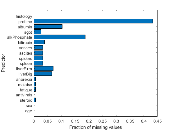
Inspect the data for missing values.

figure
barh(sum(isnan(X),1)/size(X,1))
h = gca;
h.YTick = 1:numel(VarNames) - 1;
h.YTickLabel = VarNames(2:end);
ylabel('Predictor')
xlabel('Fraction of missing values')

Most predictors have missing values, and one has nearly 45% of the missing values. Therefore, use decision trees with surrogate splits for better accuracy. Because the data set is small, training time with surrogate splits should be tolerable.

Create a classification tree template that uses surrogate splits.

rng(0,'twister') % For reproducibility
t = templateTree('surrogate','all');

Examine the data or the description of the data to see which predictors are categorical.

X(1:5,:)

ans = 5×19

   30.0000    2.0000    1.0000    2.0000    2.0000    2.0000    2.0000    1.0000    2.0000    2.0000    2.0000    2.0000    2.0000    1.0000   85.0000   18.0000    4.0000       NaN    1.0000
   50.0000    1.0000    1.0000    2.0000    1.0000    2.0000    2.0000    1.0000    2.0000    2.0000    2.0000    2.0000    2.0000    0.9000  135.0000   42.0000    3.5000       NaN    1.0000
   78.0000    1.0000    2.0000    2.0000    1.0000    2.0000    2.0000    2.0000    2.0000    2.0000    2.0000    2.0000    2.0000    0.7000   96.0000   32.0000    4.0000       NaN    1.0000
   31.0000    1.0000       NaN    1.0000    2.0000    2.0000    2.0000    2.0000    2.0000    2.0000    2.0000    2.0000    2.0000    0.7000   46.0000   52.0000    4.0000   80.0000    1.0000
   34.0000    1.0000    2.0000    2.0000    2.0000    2.0000    2.0000    2.0000    2.0000    2.0000    2.0000    2.0000    2.0000    1.0000       NaN  200.0000    4.0000       NaN    1.0000

It appears that predictors 2 through 13 are categorical, as well as predictor 19. You can confirm this inference using the data set description at UCI Machine Learning Data Repository.

List the categorical variables.

catIdx = [2:13,19];

Create a cross-validated ensemble using 50 learners and the GentleBoost algorithm.

Ensemble = fitcensemble(X,Y,'Method','GentleBoost', ...
    'NumLearningCycles',50,'Learners',t,'PredictorNames',VarNames(2:end), ...
    'LearnRate',0.1,'CategoricalPredictors',catIdx,'KFold',5);

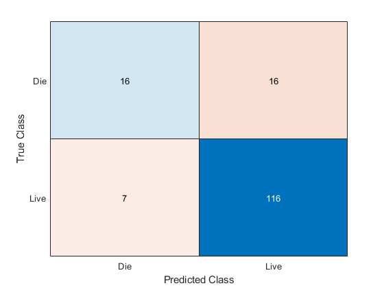
Inspect the confusion matrix to see which patients the ensemble predicts correctly.

[yFit,sFit] = kfoldPredict(Ensemble);
confusionchart(Y,yFit)

Of the 123 patient who live, the ensemble predicts correctly that 116 will live. But for the 32 patients who die of hepatitis, the ensemble only predicts correctly that about half will die of hepatitis.

There are two types of error in the predictions of the ensemble:

Predicting that the patient lives, but the patient dies
Predicting that the patient dies, but the patient lives

Suppose you believe that the first error is five times worse than the second. Create a new classification cost matrix that reflects this belief.

cost.ClassNames = ClassNames;
cost.ClassificationCosts = [0 5; 1 0];

Create a new cross-validated ensemble using cost as the misclassification cost, and inspect the resulting confusion matrix.

EnsembleCost = fitcensemble(X,Y,'Method','GentleBoost', ...
    'NumLearningCycles',50,'Learners',t,'PredictorNames',VarNames(2:end), ...
    'LearnRate',0.1,'CategoricalPredictors',catIdx,'KFold',5,'Cost',cost);
[yFitCost,sFitCost] = kfoldPredict(EnsembleCost);
confusionchart(Y,yFitCost)

As expected, the new ensemble does a better job classifying the patients who die. Somewhat surprisingly, the new ensemble also does a better job classifying the patients who live, though the result is not statistically significantly better. The results of the cross validation are random, so this result is simply a statistical fluctuation. The result seems to indicate that the classification of patients who live is not very sensitive to the cost.

References

[1] Zhou, Z.-H., and X.-Y. Liu. “On Multi-Class Cost-Sensitive Learning.” Computational Intelligence. Vol. 26, Issue 3, 2010, pp. 232–257 CiteSeerX.

[2] Breiman, L., J. H. Friedman, R. A. Olshen, and C. J. Stone. Classification and Regression Trees. Boca Raton, FL: Chapman & Hall, 1984.

[3] Zadrozny, B., J. Langford, and N. Abe. “Cost-Sensitive Learning by Cost-Proportionate Example Weighting.” Third IEEE International Conference on Data Mining, 435–442. 2003.