Main Content

classify

Classify observations using discriminant analysis

    Description

    Note

    fitcdiscr and predict are recommended over classify for training a discriminant analysis classifier and predicting labels. fitcdiscr supports cross-validation and hyperparameter optimization, and does not require you to fit the classifier every time you make a new prediction or change prior probabilities.

    class = classify(sample,training,group) classifies each row of the data in sample into one of the groups to which the data in training belongs. The groups for training are specified by group. The function returns class, which contains the assigned groups for each row of sample.

    example

    class = classify(sample,training,group,type,prior) also specifies the type of discriminant function, and prior probabilities for each group.

    [class,err,posterior,logp,coeff] = classify(___) also returns the apparent error rate (err), posterior probabilities for training observations (posterior), logarithm of the unconditional probability density for sample observations (logp), and coefficients of the boundary curves (coeff), using any of the input argument combinations in previous syntaxes.

    example

    Examples

    collapse all

    Load the fisheriris data set. Create group as a cell array of character vectors that contains the iris species.

    load fisheriris
    group = species;

    The meas matrix contains two sepal and two petal measurements for 150 irises. Randomly partition observations into a training set (trainingData) and a sample set (sampleData) with stratification, using the group information in group. Specify a 40% holdout sample for sampleData.

    rng('default') % For reproducibility
    cv = cvpartition(group,'HoldOut',0.40);
    trainInds = training(cv);
    sampleInds = test(cv);
    trainingData = meas(trainInds,:);
    sampleData = meas(sampleInds,:);

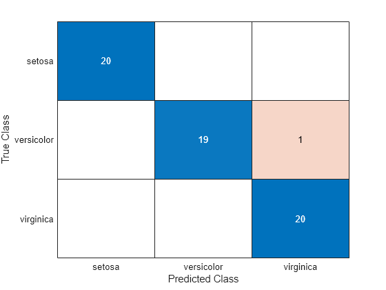
    Classify sampleData using linear discriminant analysis, and create a confusion chart from the true labels in group and the predicted labels in class.

    class = classify(sampleData,trainingData,group(trainInds));
    cm = confusionchart(group(sampleInds),class);

    Figure contains an object of type ConfusionMatrixChart.

    The classify function misclassifies one versicolor iris as virginica in the sample data set.

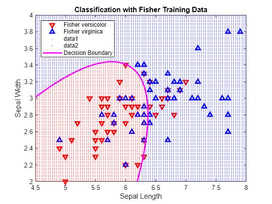
    Classify the data points in a grid of measurements (sample data) by using quadratic discriminant analysis. Then, visualize the sample data, training data, and decision boundary.

    Load the fisheriris data set. Create group as a cell array of character vectors that contains the iris species.

    load fisheriris
    group = species(51:end);

    Plot the sepal length (SL) and width (SW) measurements for the iris versicolor and virginica species.

    SL = meas(51:end,1);
    SW = meas(51:end,2);
    h1 = gscatter(SL,SW,group,'rb','v^',[],'off');
    h1(1).LineWidth = 2;
    h1(2).LineWidth = 2;
    legend('Fisher versicolor','Fisher virginica','Location','NW')
    xlabel('Sepal Length')
    ylabel('Sepal Width')

    Figure contains an axes object. The axes object with xlabel Sepal Length, ylabel Sepal Width contains 2 objects of type line. One or more of the lines displays its values using only markers These objects represent Fisher versicolor, Fisher virginica.

    Create sampleData as a numeric matrix that contains a grid of measurements. Create trainingData as a numeric matrix that contains the sepal length and width measurements for the iris versicolor and virginica species.

    [X,Y] = meshgrid(linspace(4.5,8),linspace(2,4));
    X = X(:); Y = Y(:);
    sampleData = [X Y];
    trainingData = [SL SW];

    Classify sampleData using quadratic discriminant analysis.

    [C,err,posterior,logp,coeff] = classify(sampleData,trainingData,group,'quadratic');

    Retrieve the coefficients K, L, and M for the quadratic boundary between the two classes.

    K = coeff(1,2).const;
    L = coeff(1,2).linear; 
    Q = coeff(1,2).quadratic;

    The curve that separates the two classes is defined by this equation:

    K+[x1x2]L+[x1x2]Q[x1x2]=0

    Visualize the discriminant classification.

    hold on
    h2 = gscatter(X,Y,C,'rb','.',1,'off');
    f = @(x,y) K + L(1)*x + L(2)*y + Q(1,1)*x.*x + (Q(1,2)+Q(2,1))*x.*y + Q(2,2)*y.*y;
    h3 = fimplicit(f,[4.5 8 2 4]);
    h3.Color = 'm';
    h3.LineWidth = 2;
    h3.DisplayName = 'Decision Boundary';
    hold off
    axis tight
    xlabel('Sepal Length')
    ylabel('Sepal Width')
    title('Classification with Fisher Training Data')

    Figure contains an axes object. The axes object with title Classification with Fisher Training Data, xlabel Sepal Length, ylabel Sepal Width contains 5 objects of type line, implicitfunctionline. One or more of the lines displays its values using only markers These objects represent Fisher versicolor, Fisher virginica, Decision Boundary.

    Partition a data set into sample and training data, and classify the sample data using linear discriminant analysis. Then, visualize the decision boundaries.

    Load the fisheriris data set. Create group as a cell array of character vectors that contains the iris species. Create PL and PW as numeric vectors that contain the petal length and width measurements, respectively.

    load fisheriris
    group = species;
    PL = meas(:,3);
    PW = meas(:,4);

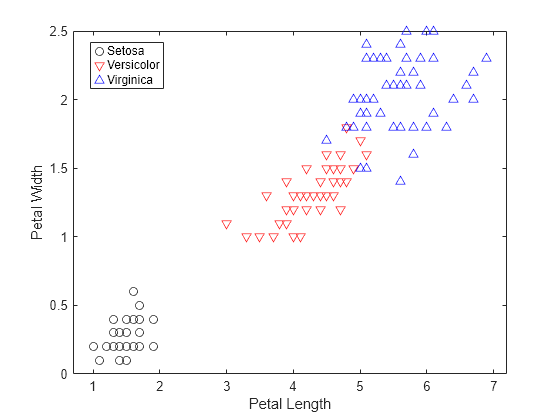
    Plot the sepal length (PL) and width (PW) measurements for the iris setosa, versicolor, and virginica species.

    h1 = gscatter(PL,PW,species,'krb','ov^',[],'off');
    legend('Setosa','Versicolor','Virginica','Location','best')
    xlabel('Petal Length')
    ylabel('Petal Width')

    Figure contains an axes object. The axes object with xlabel Petal Length, ylabel Petal Width contains 3 objects of type line. One or more of the lines displays its values using only markers These objects represent Setosa, Versicolor, Virginica.

    Randomly partition observations into a training set (trainingData) and a sample set (sampleData) with stratification, using the group information in group. Specify a 10% holdout sample for sampleData.

    rng('default') % For reproducibility
    cv = cvpartition(group,'HoldOut',0.10);
    trainInds = training(cv);
    sampleInds = test(cv);
    trainingData = [PL(trainInds) PW(trainInds)];
    sampleData = [PL(sampleInds) PW(sampleInds)];

    Classify sampleData using linear discriminant analysis.

    [class,err,posterior,logp,coeff] = classify(sampleData,trainingData,group(trainInds));

    Retrieve the coefficients K and L for the linear boundary between the second and third classes.

    K = coeff(2,3).const;  
    L = coeff(2,3).linear;

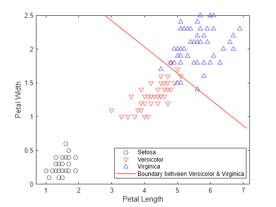
    The line that separates the second and third classes is defined by the equation K+[x1x2]L=0. Plot the boundary line between the second and third classes.

    f = @(x1,x2) K + L(1)*x1 + L(2)*x2;
    hold on
    h2 = fimplicit(f,[.9 7.1 0 2.5]);
    h2.Color = 'r';
    h2.DisplayName = 'Boundary between Versicolor & Virginica';

    Figure contains an axes object. The axes object with xlabel Petal Length, ylabel Petal Width contains 4 objects of type line, implicitfunctionline. One or more of the lines displays its values using only markers These objects represent Setosa, Versicolor, Virginica, Boundary between Versicolor & Virginica.

    Retrieve the coefficients K and L for the linear boundary between the first and second classes.

    K = coeff(1,2).const;
    L = coeff(1,2).linear;

    Plot the line that separates the first and second classes.

    f = @(x1,x2) K + L(1)*x1 + L(2)*x2;
    h3 = fimplicit(f,[.9 7.1 0 2.5]);
    hold off
    h3.Color = 'k';
    h3.DisplayName = 'Boundary between Versicolor & Setosa';
    axis tight
    title('Linear Classification with Fisher Training Data')

    Figure contains an axes object. The axes object with title Linear Classification with Fisher Training Data, xlabel Petal Length, ylabel Petal Width contains 5 objects of type line, implicitfunctionline. One or more of the lines displays its values using only markers These objects represent Setosa, Versicolor, Virginica, Boundary between Versicolor & Virginica, Boundary between Versicolor & Setosa.

    Input Arguments

    collapse all

    Sample data, specified as a numeric matrix. Each column of sample represents one variable, and each row represents one sample observation. sample must have the same number of columns as training.

    Data Types: single | double

    Training data, specified as a numeric matrix. Each column of training represents one variable, and each row represents one training observation. training must have the same number of columns as sample, and the same number of rows as group.

    Data Types: single | double

    Group names, specified as a categorical array, character array, string array, numeric vector, or cell array of character vectors. Each element in group defines the group to which the corresponding row of training belongs. group must have the same number of rows as training.

    NaN, <undefined>, empty character vector (''), empty string (""), and <missing> values in group indicate missing values. classify removes entire rows of training data corresponding to a missing group name.

    Data Types: categorical | char | string | single | double | cell

    Discriminant type, specified as one of the values in the following table.

    ValueDescription
    'linear'Fits a multivariate normal density to each group, with a pooled estimate of covariance. This option uses likelihood ratios to assign sample observations to groups.
    'quadratic'Fits multivariate normal densities with covariance estimates stratified by group. This option uses likelihood ratios to assign sample observations to groups.
    'diagLinear'Similar to 'linear', but with a diagonal covariance matrix estimate. This diagonal option is a specific example of a naive Bayes classifier, because it assumes that the variables are conditionally independent given the group label.
    'diagQuadratic'Similar to 'quadratic', but with a diagonal covariance matrix estimate. This diagonal option is a specific example of a naive Bayes classifier, because it assumes that the variables are conditionally independent given the group label.
    'mahalanobis'Uses Mahalanobis distances with stratified covariance estimates.

    Prior probabilities for each group, specified as one of the values in the following table. By default, all prior probabilities are equal to 1/K, where K is the number of groups.

    ValueDescription
    numeric vectorEach element is a group prior probability. Order the elements according to group. classify normalizes the elements so that they sum to 1.
    'empirical'The group prior probabilities are the group relative frequencies in group.
    structure

    A structure S with two fields:

    • S.group contains the group names as a variable of the same type as group.

    • S.prob contains a numeric vector of corresponding prior probabilities. classify normalizes the elements so that they sum to 1.

    prior is not used for discrimination by the Mahalanobis distance, except for the calculation of err.

    Data Types: single | double | char | string | struct

    Output Arguments

    collapse all

    Predicted class for the sample data, returned as a categorical array, character array, string array, numeric vector, or cell array of character vectors. class is of the same type as group. Each element in class contains the group to which each row of sample has been assigned.

    Data Types: categorical | char | string | single | double | cell

    Apparent error rate, returned as a nonnegative number. err is an estimate of the misclassification error rate based on the training data. It is the percentage of observations in training that are misclassified, weighted by the prior probabilities for the groups.

    Data Types: single | double

    Posterior probabilities for training observations, returned as an n-by-k numeric matrix, where n is the number of observations (rows) in training and k is the number of groups in group. The element posterior(i,j) is the posterior probability that observation i in training belongs to group j in group. If you specify type as 'mahalanobis', the function does not compute posterior.

    Data Types: single | double

    Logarithm of the unconditional probability density for sample observations, returned as a numeric vector. The predicted unconditional probability density for observation i in sample is

    P(obsi)=j=1kP(obsi | groupj)P(groupj),

    where:

    • P(obsi|groupj) is the conditional density of observation i in sample given group j in group.

    • P(groupj) is the prior probability of group j.

    • k is the number of groups.

    If you specify type as 'mahalanobis', the function does not compute logp.

    Data Types: single | double

    Coefficients of the boundary curves between pairs of groups, returned as a k-by-k structure, where k is the number of groups in group. The element coeff(i,j) contains coefficients of the boundaries between groups i and j. This table lists the coeff fields and their values.

    Field NameValue
    typeType of discriminant function, specified by type
    name1Name of the group i
    name2Name of the group j
    constConstant term of the boundary equation (K)
    linearLinear coefficients of the boundary equation (L)
    quadraticQuadratic coefficient matrix of the boundary equation (Q). The structure does not include this field when you specify type as 'linear' or 'diagLinear'.
    • If you specify type as 'linear' or 'diagLinear', the function classifies a row x from sample into group i (instead of group j) when 0 < K + x*L.

    • If you specify type as 'quadratic', 'diagQuadratic', or 'mahalanobis', the function classifies a row x from sample into group i (instead of group j) when 0 < K + x*L + x*Q*x'.

    Alternative Functionality

    The fitcdiscr function also performs discriminant analysis. You can train a classifier by using the fitcdiscr function and predict labels of new data by using the predict function. The fitcdiscr function supports cross-validation and hyperparameter optimization, and does not require you to fit the classifier every time you make a new prediction or change prior probabilities.

    References

    [1] Krzanowski, Wojtek. J. Principles of Multivariate Analysis: A User's Perspective. NY: Oxford University Press, 1988.

    [2] Seber, George A. F. Multivariate Observations. NJ: John Wiley & Sons, Inc., 1984.

    Version History

    Introduced before R2006a
    Go to top of page