Main Content

cluster

Construct agglomerative clusters from linkages

Description

T = cluster(Z,'Cutoff',C) defines clusters from an agglomerative hierarchical cluster tree Z. The input Z is the output of the linkage function for an input data matrix X. cluster cuts Z into clusters, using C as a threshold for the inconsistency coefficients (or inconsistent values) of nodes in the tree. The output T contains cluster assignments of each observation (row of X).

example

T = cluster(Z,'Cutoff',C,'Depth',D) evaluates inconsistent values by looking to a depth D below each node.

example

T = cluster(Z,'Cutoff',C,'Criterion',criterion) uses either 'inconsistent' (default) or 'distance' as the criterion for defining clusters. criterion must be less than C for cluster to define clusters.

example

T = cluster(Z,'MaxClust',N) defines a maximum of N clusters using 'distance' as the criterion for defining clusters.

Examples

collapse all

Perform agglomerative clustering on randomly generated data by evaluating inconsistent values to a depth of four below each node.

Randomly generate the sample data.

rng('default'); % For reproducibility
X = [(randn(20,2)*0.75)+1;
    (randn(20,2)*0.25)-1];

Create a scatter plot of the data.

scatter(X(:,1),X(:,2));
title('Randomly Generated Data');

Figure contains an axes object. The axes object with title Randomly Generated Data contains an object of type scatter.

Create a hierarchical cluster tree using the ward linkage method.

Z = linkage(X,'ward');

Create a dendrogram plot of the data.

dendrogram(Z)

Figure contains an axes object. The axes object contains 29 objects of type line.

The scatter plot and the dendrogram plot seem to show two clusters in the data.

Cluster the data using a threshold of 3 for the inconsistency coefficient and looking to a depth of 4 below each node. Plot the resulting clusters.

T = cluster(Z,'cutoff',3,'Depth',4);
gscatter(X(:,1),X(:,2),T)

Figure contains an axes object. The axes object contains 2 objects of type line. One or more of the lines displays its values using only markers These objects represent 1, 2.

cluster identifies two clusters in the data.

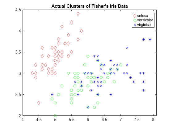
Perform agglomerative clustering on the fisheriris data set using 'distance' as the criterion for defining clusters. Visualize the cluster assignments of the data.

Load the fisheriris data set.

load fisheriris

Visualize a 2-D scatter plot of the data using species as the grouping variable. Specify marker colors and marker symbols for the three different species.

gscatter(meas(:,1),meas(:,2),species,'rgb','do*')
title("Actual Clusters of Fisher's Iris Data")

Figure contains an axes object. The axes object with title Actual Clusters of Fisher's Iris Data contains 3 objects of type line. One or more of the lines displays its values using only markers These objects represent setosa, versicolor, virginica.

Create a hierarchical cluster tree using the 'average' method and the 'chebychev' metric.

Z = linkage(meas,'average','chebychev');

Cluster the data using a threshold of 1.5 for the 'distance' criterion.

T = cluster(Z,'cutoff',1.5,'Criterion','distance')
T = 150×1

     2
     2
     2
     2
     2
     2
     2
     2
     2
     2
      ⋮

T contains numbers that correspond to the cluster assignments. Find the number of classes that cluster identifies.

length(unique(T))
ans = 3

cluster identifies three classes for the specified values of cutoff and Criterion.

Visualize a 2-D scatter plot of the clustering results using T as the grouping variable. Specify marker colors and marker symbols for the three different classes.

gscatter(meas(:,1),meas(:,2),T,'rgb','do*')
title("Cluster Assignments of Fisher's Iris Data")

Figure contains an axes object. The axes object with title Cluster Assignments of Fisher's Iris Data contains 3 objects of type line. One or more of the lines displays its values using only markers These objects represent 1, 2, 3.

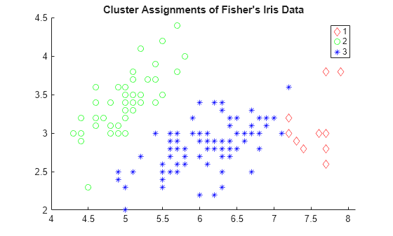
Clustering correctly identifies the setosa class (class 2) as belonging to a distinct cluster, but poorly distinguishes between the versicolor and virginica classes (classes 1 and 3, respectively). Note that the scatter plot labels the classes using the numbers contained in T.

Find a maximum of three clusters in the fisheriris data set and compare cluster assignments of the flowers to their known classification.

Load the sample data.

load fisheriris

Create a hierarchical cluster tree using the 'average' method and the 'chebychev' metric.

Z = linkage(meas,'average','chebychev');

Find a maximum of three clusters in the data.

T = cluster(Z,'maxclust',3);

Create a dendrogram plot of Z. To see the three clusters, use 'ColorThreshold' with a cutoff halfway between the third-from-last and second-from-last linkages.

cutoff = median([Z(end-2,3) Z(end-1,3)]);
dendrogram(Z,'ColorThreshold',cutoff)

Figure contains an axes object. The axes object contains 29 objects of type line.

Display the last two rows of Z to see how the three clusters are combined into one. linkage combines the 293rd (blue) cluster with the 297th (red) cluster to form the 298th cluster with a linkage of 1.7583. linkage then combines the 296th (green) cluster with the 298th cluster.

lastTwo = Z(end-1:end,:)
lastTwo = 2×3

  293.0000  297.0000    1.7583
  296.0000  298.0000    3.4445

See how the cluster assignments correspond to the three species. For example, one of the clusters contains 50 flowers of the second species and 40 flowers of the third species.

crosstab(T,species)
ans = 3×3

     0     0    10
     0    50    40
    50     0     0

Randomly generate sample data with 20,000 observations.

rng('default') % For reproducibility
X = rand(20000,3);

Create a hierarchical cluster tree using the ward linkage method. In this case, the 'SaveMemory' option of the clusterdata function is set to 'on' by default. In general, specify the best value for 'SaveMemory' based on the dimensions of X and the available memory.

Z = linkage(X,'ward');

Cluster the data into a maximum of four groups and plot the result.

c = cluster(Z,'Maxclust',4);
scatter3(X(:,1),X(:,2),X(:,3),10,c)

Figure contains an axes object. The axes object contains an object of type scatter.

cluster identifies four groups in the data.

Input Arguments

collapse all

Agglomerative hierarchical cluster tree that is the output of the linkage function, specified as a numeric matrix. For an input data matrix X with m rows (or observations), linkage returns an (m – 1)-by-3 matrix Z. For an explanation of how linkage creates the cluster tree, see Z.

Example: Z = linkage(X), where X is an input data matrix

Data Types: single | double

Threshold for defining clusters, specified as a positive scalar or a vector of positive scalars. cluster uses C as a threshold for either the heights or the inconsistency coefficients of nodes, depending on the criterion for defining clusters in a hierarchical cluster tree.

  • If the criterion for defining clusters is 'distance', then cluster groups all leaves at or below a node into a cluster, provided that the height of the node is less than C.

  • If the criterion for defining clusters is 'inconsistent', then the inconsistent values of a node and all its subnodes must be less than C for cluster to group them into a cluster. cluster begins from the root of the cluster tree Z and steps down through the tree until it encounters a node whose inconsistent value is less than the threshold C, and whose subnodes (or descendants) have inconsistent values less than C. Then cluster groups all leaves at or below the node into a cluster (or a singleton if the node itself is a leaf). cluster follows every branch in the tree until all leaf nodes are in clusters.

Example: cluster(Z,'Cutoff',0.5)

Data Types: single | double

Depth for computing inconsistent values, specified as a numeric scalar. cluster evaluates inconsistent values by looking to a depth D below each node.

Example: cluster(Z,'Cutoff',0.5,'Depth',3)

Data Types: single | double

Criterion for defining clusters, specified as 'inconsistent' or 'distance'.

If the criterion for defining clusters is 'distance', then cluster groups all leaves at or below a node into a cluster (or a singleton if the node itself is a leaf), provided that the height of the node is less than C. The height of a node in a tree represents the distance between the two subnodes that are merged at that node. Specifying 'distance' results in clusters that correspond to a horizontal slice of the dendrogram plot of Z.

If the criterion for defining clusters is 'inconsistent', then cluster groups a node and all its subnodes into a cluster, provided that the inconsistency coefficients (or inconsistent values) of the node and subnodes are less than C. Specifying 'inconsistent' is equivalent to cluster(Z,'Cutoff',C).

Example: cluster(Z,'Cutoff',0.5,'Criterion','distance')

Data Types: char | string

Maximum number of clusters to form, specified as a positive integer or a vector of positive integers. cluster constructs a maximum of N clusters, using 'distance' as the criterion for defining clusters. The height of each node in the tree represents the distance between the two subnodes merged at that node. cluster finds the smallest height at which a horizontal cut through the tree will leave N or fewer clusters. See Specify Arbitrary Clusters for more details.

Example: cluster(Z,'MaxClust',5)

Data Types: single | double

Output Arguments

collapse all

Cluster assignment, returned as a numeric vector or matrix. For the (m – 1)-by-3 hierarchical cluster tree Z (the output of linkage given input X), T contains the cluster assignments of the m rows (observations) of X.

The size of T depends on the corresponding size of C or N.

  • If C is a positive scalar, then T is a vector of length m.

  • If N is a positive integer, then T is a vector of length m.

  • If C is a length l vector of positive scalars, then T is an m-by-l matrix with one column per value in C.

  • If N is a length l vector of positive integers, then T is an m-by-l matrix with one column per value in N.

Alternative Functionality

If you have an input data matrix X, you can use clusterdata to perform agglomerative clustering and return cluster indices for each observation (row) in X. The clusterdata function performs all the necessary steps for you, so you do not need to execute the pdist, linkage, and cluster functions separately.

Version History

Introduced before R2006a