linkage
Agglomerative hierarchical cluster tree
Syntax
Description
Examples
Randomly generate sample data with 20,000 observations.
rng(0,"twister") % For reproducibility
X = rand(20000,3);
Create a hierarchical cluster tree using the ward linkage method. In this case, the SaveMemory option of the clusterdata function is set to "on" by default. In general, specify the best value for SaveMemory based on the dimensions of X and the available memory.
Z = linkage(X,"ward");Cluster the data into a maximum of four groups and plot the result.
c = cluster(Z,MaxClust=4);
scatter3(X(:,1),X(:,2),X(:,3),10,c)

cluster identifies four groups in the data.
Find a maximum of three clusters in the fisheriris data set and compare cluster assignments of the flowers to their known classification.
Load the sample data.
load fisheririsCreate a hierarchical cluster tree using the "average" method and the "chebychev" metric.
Z = linkage(meas,"average","chebychev");
Find a maximum of three clusters in the data.
T = cluster(Z,MaxClust=3);
Create a dendrogram plot of Z. To see the three clusters, use ColorThreshold with a cutoff halfway between the third-from-last and second-from-last linkages.
cutoff = median([Z(end-2,3) Z(end-1,3)]);
dendrogram(Z,ColorThreshold=cutoff,ShowCut=true)

Display the last two rows of Z to see how the three clusters are combined into one. linkage combines the 293rd (orange) cluster with the 297th (blue) cluster to form the 298th cluster with a linkage of 1.7583. linkage then combines the 296th (red) cluster with the 298th cluster.
lastTwo = Z(end-1:end,:)
lastTwo = 2×3

  293.0000  297.0000    1.7583
  296.0000  298.0000    3.4445
The cluster assignments correspond to the three species. For example, one of the clusters contains 50 flowers of the second species and 40 flowers of the third species.
crosstab(T,species)
ans = 3×3

     0     0    10
     0    50    40
    50     0     0
Load the examgrades data set.
load examgradesCreate a hierarchical tree using linkage. Use the 'single' method and the Minkowski metric with an exponent of 3.
Z = linkage(grades,'single',{'minkowski',3});
Observe the 25th clustering step.
Z(25,:)
ans = 1×3

   86.0000  137.0000    4.5307
linkage combines the 86th observation and the 137th cluster to form a cluster of index , where 120 is the total number of observations in grades and 25 is the row number in Z. The shortest distance between the 86th observation and any of the points in the 137th cluster is 4.5307.
Create an agglomerative hierarchical cluster tree using a dissimilarity matrix.
Take a dissimilarity matrix X and convert it to a vector form that linkage accepts by using squareform.
X = [0 1 2 3; 1 0 4 5; 2 4 0 6; 3 5 6 0];
y = squareform(X);
Create a cluster tree using linkage with the 'complete' method of calculating the distance between clusters. The first two columns of Z show how linkage combines clusters. The third column of Z gives the distance between clusters.
Z = linkage(y,'complete')Z = 3×3
1 2 1
3 5 4
4 6 6
Create a dendrogram plot of Z. The x-axis corresponds to the leaf nodes of the tree, and the y-axis corresponds to the linkage distances between clusters.
dendrogram(Z)
Input Arguments
Output Arguments
More About
Tips
Computing
linkage(y)can be slow whenyis a vector representation of the distance matrix. For the'centroid','median', and'ward'methods,linkagechecks whetheryis a Euclidean distance. Avoid this time-consuming check by passing inXinstead ofy.The
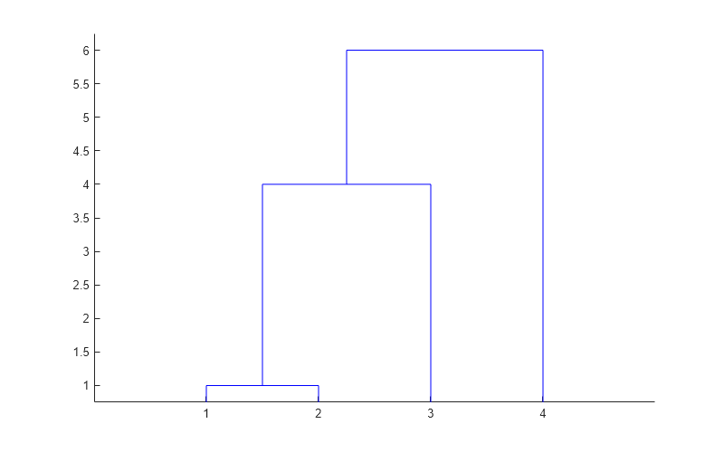
'centroid'and'median'methods can produce a cluster tree that is not monotonic. This result occurs when the distance from the union of two clusters, r and s, to a third cluster is less than the distance between r and s. In this case, in a dendrogram drawn with the default orientation, the path from a leaf to the root node takes some downward steps. To avoid this result, use another method. This figure shows a nonmonotonic cluster tree.
In this case, cluster 1 and cluster 3 are joined into a new cluster, and the distance between this new cluster and cluster 2 is less than the distance between cluster 1 and cluster 3. The result is a nonmonotonic tree.
You can provide the output
Zto other functions includingdendrogramto display the tree,clusterto assign points to clusters,inconsistentto compute inconsistent measures, andcophenetto compute the cophenetic correlation coefficient.
Version History
Introduced before R2006a
See Also
cluster | clusterdata | cophenet | dendrogram | inconsistent | kmeans | pdist | silhouette | squareform