Improving Classification Trees and Regression Trees
You can tune trees by setting name-value pairs in fitctree and fitrtree. The remainder of this section
describes how to determine the quality of a tree, how to decide which name-value pairs
to set, and how to control the size of a tree.
Examining Resubstitution Error
Resubstitution error is the difference between the response training data and the predictions the tree makes of the response based on the input training data. If the resubstitution error is high, you cannot expect the predictions of the tree to be good. However, having low resubstitution error does not guarantee good predictions for new data. Resubstitution error is often an overly optimistic estimate of the predictive error on new data.
Classification Tree Resubstitution Error
This example shows how to examine the resubstitution error of a classification tree.
Load Fisher's iris data.
load fisheririsTrain a default classification tree using the entire data set.
Mdl = fitctree(meas,species);
Examine the resubstitution error.
resuberror = resubLoss(Mdl)
resuberror =
0.0200
The tree classifies nearly all the Fisher iris data correctly.
Cross Validation
To get a better sense of the predictive accuracy of your tree for new data, cross validate the tree. By default, cross validation splits the training data into 10 parts at random. It trains 10 new trees, each one on nine parts of the data. It then examines the predictive accuracy of each new tree on the data not included in training that tree. This method gives a good estimate of the predictive accuracy of the resulting tree, since it tests the new trees on new data.
Cross Validate a Regression Tree
This example shows how to examine the resubstitution and cross-validation accuracy of a regression tree for predicting mileage based on the carsmall data.
Load the carsmall data set. Consider acceleration, displacement, horsepower, and weight as predictors of MPG.
load carsmall
X = [Acceleration Displacement Horsepower Weight];
Grow a regression tree using all of the observations.
rtree = fitrtree(X,MPG);
Compute the in-sample error.
resuberror = resubLoss(rtree)
resuberror =
4.7188
The resubstitution loss for a regression tree is the mean-squared error. The resulting value indicates that a typical predictive error for the tree is about the square root of 4.7, or a bit over 2.
Estimate the cross-validation MSE.
rng 'default';
cvrtree = crossval(rtree);
cvloss = kfoldLoss(cvrtree)
cvloss = 23.5706
The cross-validated loss is almost 25, meaning a typical predictive error for the tree on new data is about 5. This demonstrates that cross-validated loss is usually higher than simple resubstitution loss.
Choose Split Predictor Selection Technique
The standard CART algorithm tends to select continuous predictors that have many levels. Sometimes, such a selection can be spurious and can also mask more important predictors that have fewer levels, such as categorical predictors. That is, the predictor-selection process at each node is biased. Also, standard CART tends to miss the important interactions between pairs of predictors and the response.
To mitigate selection bias and increase detection of important interactions, you
can specify usage of the curvature or interaction tests using the
'PredictorSelection' name-value pair argument. Using the
curvature or interaction test has the added advantage of producing better predictor
importance estimates than standard CART.
This table summarizes the supported predictor-selection techniques.
| Technique | 'PredictorSelection'
Value | Description | Training speed | When to specify |
|---|---|---|---|---|
| Standard CART [1] | Default |
Selects the split predictor that maximizes the split-criterion gain over all possible splits of all predictors. | Baseline for comparison |
Specify if any of these conditions are true:
|
| Curvature test [2][3] | 'curvature' | Selects the split predictor that minimizes the p-value of chi-square tests of independence between each predictor and the response. | Comparable to standard CART |
Specify if any of these conditions are true:
|
| Interaction test [3] | 'interaction-curvature' | Chooses the split predictor that minimizes the p-value of chi-square tests of independence between each predictor and the response (that is, conducts curvature tests), and that minimizes the p-value of a chi-square test of independence between each pair of predictors and response. | Slower than standard CART, particularly when data set contains many predictor variables. |
Specify if any of these conditions are true:
|
For more details on predictor selection techniques:
For classification trees, see
PredictorSelectionand Node Splitting Rules.For regression trees, see
PredictorSelectionand Node Splitting Rules.
Control Depth or “Leafiness”
When you grow a decision tree, consider its simplicity and predictive power. A deep tree with many leaves is usually highly accurate on the training data. However, the tree is not guaranteed to show a comparable accuracy on an independent test set. A leafy tree tends to overtrain (or overfit), and its test accuracy is often far less than its training (resubstitution) accuracy. In contrast, a shallow tree does not attain high training accuracy. But a shallow tree can be more robust — its training accuracy could be close to that of a representative test set. Also, a shallow tree is easy to interpret. If you do not have enough data for training and test, estimate tree accuracy by cross validation.
fitctree and fitrtree have three name-value pair arguments that control the depth
of resulting decision trees:
MaxNumSplits— The maximal number of branch node splits isMaxNumSplitsper tree. Set a large value forMaxNumSplitsto get a deep tree. The default issize(X,1) – 1.MinLeafSize— Each leaf has at leastMinLeafSizeobservations. Set small values ofMinLeafSizeto get deep trees. The default is1.MinParentSize— Each branch node in the tree has at leastMinParentSizeobservations. Set small values ofMinParentSizeto get deep trees. The default is10.
If you specify MinParentSize and
MinLeafSize, the learner uses the setting that yields trees with
larger leaves (i.e., shallower trees):
MinParent =
                    max(MinParentSize,2*MinLeafSize)
If you supply MaxNumSplits, the software splits a tree until
one of the three splitting criteria is satisfied.
For an alternative method of controlling the tree depth, see Pruning.
Select Appropriate Tree Depth
This example shows how to control the depth of a decision tree, and how to choose an appropriate depth.
Load the ionosphere data.
load ionosphereGenerate an exponentially spaced set of values from 10 through 100 that represent the minimum number of observations per leaf node.
leafs = logspace(1,2,10);
Create cross-validated classification trees for the ionosphere data. Specify to grow each tree using a minimum leaf size in leafs.
rng('default')
N = numel(leafs);
err = zeros(N,1);
for n=1:N
    t = fitctree(X,Y,'CrossVal','On',...
        'MinLeafSize',leafs(n));
    err(n) = kfoldLoss(t);
end
plot(leafs,err);
xlabel('Min Leaf Size');
ylabel('cross-validated error');
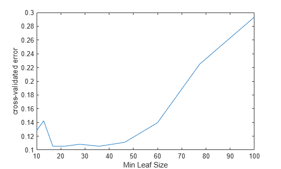
The best leaf size is between about 20 and 50 observations per leaf.
Compare the near-optimal tree with at least 40 observations per leaf with the default tree, which uses 10 observations per parent node and 1 observation per leaf.
DefaultTree = fitctree(X,Y);
view(DefaultTree,'Mode','Graph')
OptimalTree = fitctree(X,Y,'MinLeafSize',40);
view(OptimalTree,'mode','graph')

resubOpt = resubLoss(OptimalTree);
lossOpt = kfoldLoss(crossval(OptimalTree));
resubDefault = resubLoss(DefaultTree);
lossDefault = kfoldLoss(crossval(DefaultTree));
resubOpt,resubDefault,lossOpt,lossDefault
resubOpt =
0.0883
resubDefault =
0.0114
lossOpt =
0.1054
lossDefault =
0.1054
The near-optimal tree is much smaller and gives a much higher resubstitution error. Yet, it gives similar accuracy for cross-validated data.
Pruning
Pruning optimizes tree depth (leafiness) by merging leaves on the same tree branch. Control Depth or “Leafiness” describes one method for selecting the optimal depth for a tree. Unlike in that section, you do not need to grow a new tree for every node size. Instead, grow a deep tree, and prune it to the level you choose.
Prune a tree at the command line using the prune method (classification) or prune method (regression). Alternatively, prune a tree interactively
using the tree viewer:
view(tree,'mode','graph')
To prune a tree, the tree must contain a pruning sequence. By default, both
fitctree and fitrtree calculate a pruning sequence for a tree during
construction. If you construct a tree with the 'Prune' name-value
pair set to 'off', or if you prune a tree to a smaller level, the
tree does not contain the full pruning sequence. Generate the full pruning sequence
with the prune method (classification) or
prune method (regression).
How Decision Trees Create a Pruning Sequence
As explained in Growing Decision Trees, fitctree and
fitrtree create decision trees by minimizing an
optimization criterion for the splits: mean squared error for regression, or a
measure of impurity for classification. The risk
r(t) of a node t is the
optimization criterion e(t) multiplied by
the probability of the node:
r(t) = P(t)e(t).
The risk for the entire tree is the sum of the risks over the leaf nodes in the tree.
In order to not overtrain a tree, the software can add the number of leaf nodes as a penalty term, multiplied by a constant ɑ. So the risk measure for the tree is
where L is the set of leaf nodes of the tree.
Pruning a tree is the process of merging two leaf nodes that split from one parent node back to the parent node, causing the parent node to become a leaf node. You can prune a tree manually, as shown in the next section. Pruning merges leaves that together have higher risk than the parent node alone. As ɑ increases from 0, more leaves of the optimal tree merge into their parent nodes, until at a high enough ɑ, the tree has just one node. For a parent node p with leaves s and t, the total risk of the tree decreases if
r(p) < r(s) + r(t) + ɑ.
The software stores the sequence of ɑ values that cause the
nodes to merge in the PruneAlpha property of the tree, and
the list of the pruning levels of each node in the tree in the
PruneList property. The PruneList
property has entries from 0 (no pruning) to M, where
M is the number of levels from the root node to the
farthest leaf node in the tree.
Prune a Classification Tree
This example creates a classification tree for the ionosphere data, and prunes it to a good level.
Load the ionosphere data:
load ionosphereConstruct a default classification tree for the data:
tree = fitctree(X,Y);
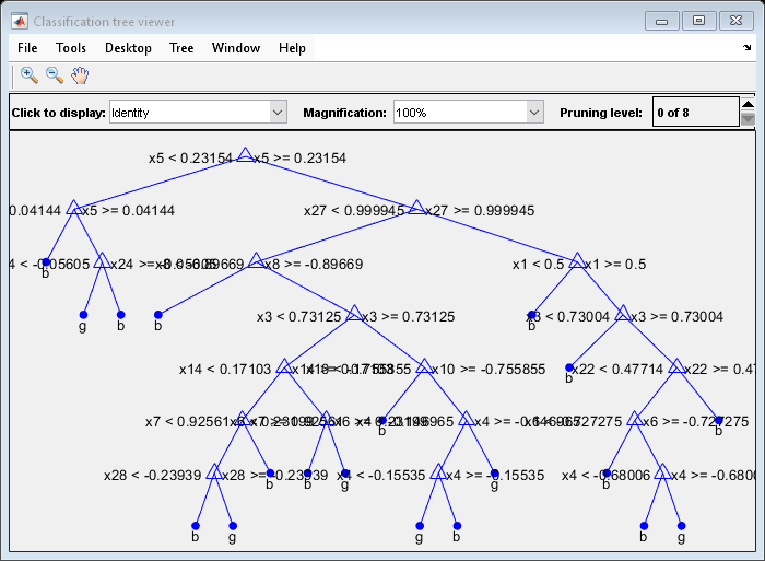
View the tree in the interactive viewer:
view(tree,'Mode','Graph')

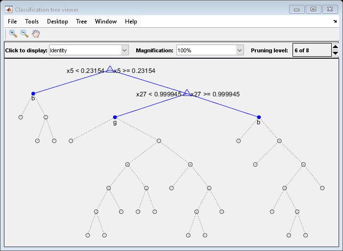
Find the optimal pruning level by minimizing cross-validated loss:
[~,~,~,bestlevel] = cvLoss(tree,...
    'SubTrees','All','TreeSize','min')
bestlevel =
6
Prune the tree to level 6:
view(tree,'Mode','Graph','Prune',6)
Alternatively, use the interactive window to prune the tree.
The pruned tree is the same as the near-optimal tree in the "Select Appropriate Tree Depth" example.
Set 'TreeSize' to 'SE' (default) to find the maximal pruning level for which the tree error does not exceed the error from the best level plus one standard deviation:
[~,~,~,bestlevel] = cvLoss(tree,'SubTrees','All')
bestlevel =
6
In this case the level is the same for either setting of 'TreeSize'.
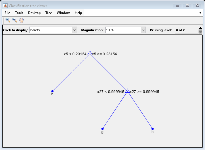
Prune the tree to use it for other purposes:
tree = prune(tree,'Level',6);
view(tree,'Mode','Graph')
References
[1] Breiman, L., J. H. Friedman, R. A. Olshen, and C. J. Stone. Classification and Regression Trees. Boca Raton, FL: Chapman & Hall, 1984.
[2] Loh, W.Y. and Y.S. Shih. “Split Selection Methods for Classification Trees.” Statistica Sinica, Vol. 7, 1997, pp. 815–840.
[3] Loh, W.Y. “Regression Trees with Unbiased Variable Selection and Interaction Detection.” Statistica Sinica, Vol. 12, 2002, pp. 361–386.
See Also
fitctree | fitrtree | ClassificationTree | RegressionTree | predict (CompactRegressionTree) | predict (CompactClassificationTree) | prune (ClassificationTree) | prune (RegressionTree)