Main Content

mnrval

(Not recommended) Multinomial logistic regression values

mnrval is not recommended. Instead, use fitmnr to create a MultinomialRegression model object and then use the predict object function. (since R2023a) For more information see Version History.

Description

example

pihat = mnrval(B,X) returns the predicted probabilities for the multinomial logistic regression model with predictors, X, and the coefficient estimates, B.

pihat is an n-by-k matrix of predicted probabilities for each multinomial category. B is the vector or matrix that contains the coefficient estimates returned by mnrfit. And X is an n-by-p matrix which contains n observations for p predictors.

Note

mnrval automatically includes a constant term in all models. Do not enter a column of 1s in X.

example

[pihat,dlow,dhi] = mnrval(B,X,stats) also returns 95% error bounds on the predicted probabilities, pihat, using the statistics in the structure, stats, returned by mnrfit.

The lower and upper confidence bounds for pihat are pihat minus dlow and pihat plus dhi, respectively. Confidence bounds are nonsimultaneous and only apply to the fitted curve, not to new observations.

[pihat,dlow,dhi] = mnrval(B,X,stats,Name,Value) returns the predicted probabilities and 95% error bounds on the predicted probabilities pihat, with additional options specified by one or more Name,Value pair arguments.

For example, you can specify the model type, link function, and the type of probabilities to return.

yhat = mnrval(B,X,ssize) returns the predicted category counts for sample sizes, ssize.

example

[yhat,dlow,dhi] = mnrval(B,X,ssize,stats) also computes 95% error bounds on the predicted counts yhat, using the statistics in the structure, stats, returned by mnrfit.

The lower and upper confidence bounds for yhat are yhat minus dlo and yhat plus dhi, respectively. Confidence bounds are nonsimultaneous and they apply to the fitted curve, not to new observations.

example

[yhat,dlow,dhi] = mnrval(B,X,ssize,stats,Name,Value) returns the predicted category counts and 95% error bounds on the predicted counts yhat, with additional options specified by one or more Name,Value pair arguments.

For example, you can specify the model type, link function, and the type of predicted counts to return.

Examples

collapse all

Fit a multinomial regression for nominal outcomes and estimate the category probabilities.

Load the sample data.

load fisheriris

The column vector, species, consists of iris flowers of three different species: setosa, versicolor, virginica. The double matrix meas consists of four types of measurements on the flowers, the length and width of sepals and petals in centimeters, respectively.

Define the nominal response variable.

sp = nominal(species);
sp = double(sp);

Now in sp, 1, 2, and 3 indicate the species setosa, versicolor, and virginica, respectively.

Fit a nominal model to estimate the species using the flower measurements as the predictor variables.

[B,dev,stats] = mnrfit(meas,sp);

Estimate the probability of being a certain kind of species for an iris flower having the measurements (6.3, 2.8, 4.9, 1.7).

x = [6.3, 2.8, 4.9, 1.7];
pihat = mnrval(B,x);
pihat
pihat = 1×3

         0    0.3977    0.6023

The probability of an iris flower having the measurements (6.3, 2.8, 4.9, 1.7) being a setosa is 0, a versicolor is 0.3977, and a virginica is 0.6023.

Fit a multinomial regression model for categorical responses with natural ordering among categories. Then estimate the upper and lower confidence bounds for the category probability estimates.

Load the sample data and define the predictor variables.

load('carbig.mat')
X = [Acceleration Displacement Horsepower Weight];

The predictor variables are the acceleration, engine displacement, horsepower, and the weight of the cars. The response variable is miles per gallon (MPG).

Create an ordinal response variable categorizing MPG into four levels from 9 to 48 mpg.

miles = ordinal(MPG,{'1','2','3','4'},[],[9,19,29,39,48]);
miles = double(miles);

Now in miles, 1 indicates the cars with miles per gallon from 9 to 19, and 2 indicates the cars with miles per gallon from 20 to 29. Similarly, 3 and 4 indicate the cars with miles per gallon from 30 to 39 and 40 to 48, respectively.

Fit a multinomial regression model for the response variable miles. For an ordinal model, the default 'link' is logit and the default 'interactions' is 'off'.

[B,dev,stats] = mnrfit(X,miles,'model','ordinal');

Compute the probability estimates and 95% error bounds for probability confidence intervals for miles per gallon of a car with x = (12, 113, 110, 2670).

x = [12,113,110,2670];
[pihat,dlow,hi] = mnrval(B,x,stats,'model','ordinal');
pihat
pihat = 1×4

    0.0615    0.8426    0.0932    0.0027

Calculate the confidence bounds for the category probability estimates.

LL = pihat - dlow;
UL = pihat + hi;
[LL;UL]
ans = 2×4

    0.0073    0.7829    0.0283   -0.0003
    0.1157    0.9022    0.1580    0.0057

Fit a multinomial regression for nominal outcomes and estimate the category counts.

Load the sample data.

load fisheriris

The column vector, species, consists of iris flowers of three different species: setosa, versicolor, and virginica. The double matrix meas consists of four types of measurements on the flowers, the length and width of sepals and petals in centimeters, respectively.

Define the nominal response variable.

sp = nominal(species);
sp = double(sp);

Now in sp, 1, 2, and 3 indicate the species setosa, versicolor, and virginica, respectively.

Fit a nominal model to estimate the species based on the flower measurements.

[B,dev,stats] = mnrfit(meas,sp);

Estimate the number in each species category for a sample of 100 iris flowers all with the measurements (6.3, 2.8, 4.9, 1.7).

x = [6.3, 2.8, 4.9, 1.7];
yhat = mnrval(B,x,18)
yhat = 1×3

         0    7.1578   10.8422

Estimate the error bounds for the counts.

[yhat,dlow,hi] = mnrval(B,x,18,stats,'model','nominal');

Calculate the confidence bounds for the category probability estimates.

LL = yhat - dlow;
UL = yhat + hi;
[LL;UL]
ans = 2×3

         0    3.3019    6.9863
         0   11.0137   14.6981

Create sample data with one predictor variable and a categorical response variable with three categories.

x = [-3 -2 -1 0 1 2 3]';
Y = [1 11 13; 2 9 14; 6 14 5; 5 10 10;...
		 5 14 6; 7 13 5; 8 11 6];
[Y x]
ans = 7×4

     1    11    13    -3
     2     9    14    -2
     6    14     5    -1
     5    10    10     0
     5    14     6     1
     7    13     5     2
     8    11     6     3

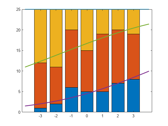
There are observations on seven different values of the predictor variable x . The response variable Y has three categories and the data shows how many of the 25 individuals are in each category of Y for each observation of x. For example, when x is -3, 1 of 25 individuals is observed in category 1, 11 observed in category 2, and 13 observed in category 3. Similarly, when x is 1, 5 of the individuals are observed in category 1, 14 are observed in category 2, and 6 are observed in category 3.

Plot the number in each category versus the x values, on a stacked bar graph.

bar(x,Y,'stacked'); 
ylim([0 25]);

Fit a nominal model for the individual response category probabilities, with separate slopes on the single predictor variable, x, for each category.

betaHatNom = mnrfit(x,Y,'model','nominal',...
    'interactions','on')
betaHatNom = 2×2

   -0.6028    0.3832
    0.4068    0.1948

The first row of betaHatOrd contains the intercept terms for the first two response categories. The second row contains the slopes. mnrfit accepts the third category as the reference category and hence assumes the coefficients for the third category are zero.

Compute the predicted probabilities for the three response categories.

xx = linspace(-4,4)';
piHatNom = mnrval(betaHatNom,xx,'model','nominal',...
    'interactions','on');

The probability of being in the third category is simply 1 - P(y = 1) - P(y = 2).

Plot the estimated cumulative number in each category on the bar graph.

line(xx,cumsum(25*piHatNom,2),'LineWidth',2);

The cumulative probability for the third category is always 1.

Now, fit a "parallel" ordinal model for the cumulative response category probabilities, with a common slope on the single predictor variable, x, across all categories:

betaHatOrd = mnrfit(x,Y,'model','ordinal',...
    'interactions','off')
betaHatOrd = 3×1

   -1.5001
    0.7266
    0.2642

The first two elements of betaHatOrd are the intercept terms for the first two response categories. The last element of betaHatOrd is the common slope.

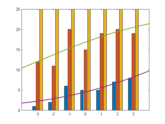
Compute the predicted cumulative probabilities for the first two response categories. The cumulative probability for the third category is always 1.

piHatOrd = mnrval(betaHatOrd,xx,'type','cumulative',...
    'model','ordinal','interactions','off');

Plot the estimated cumulative number on the bar graph of the observed cumulative number.

figure()
bar(x,cumsum(Y,2),'grouped'); 
ylim([0 25]);
line(xx,25*piHatOrd,'LineWidth',2);

Input Arguments

collapse all

Coefficient estimates for the multinomial logistic regression model, specified as a vector or matrix returned by mnrfit. It is a vector or matrix depending on the model and interactions.

Example: B = mnrfit(X,y); pihat = mnrval(B,X)

Data Types: single | double

Sample data on predictors, specified as an n-by-p. X contains n observations for p predictors.

Note

mnrval automatically includes a constant term in all models. Do not enter a column of 1s in X.

Example: pihat = mnrval(B,X)

Data Types: single | double

Model statistics, specified as a structure returned by mnrfit. You must use the stats input argument in mnrval to compute the lower and upper error bounds on the category probabilities and counts.

Example: [B,dev,stats] = mnrfit(X,y);[pihat,dlo,dhi] = mnrval(B,X,stats)

Sample sizes to return the number of items in response categories for each combination of the predictor variables, specified as an n-by-1 column vector of positive integers.

For example, for a response variable having three categories, if an observation of the number of individuals in each category is y1, y2, and y3, respectively, then the sample size, m, for that observation is m = y1 + y2 + y3.

If the sample sizes for n observations are in vector sample, then you can enter the sample sizes as follows.

Example: yhat = mnrval(B,X,sample)

Data Types: single | double

Name-Value Arguments

Specify optional pairs of arguments as Name1=Value1,...,NameN=ValueN, where Name is the argument name and Value is the corresponding value. Name-value arguments must appear after other arguments, but the order of the pairs does not matter.

Before R2021a, use commas to separate each name and value, and enclose Name in quotes.

Example: 'model','ordinal','link','probit','type','cumulative' specifies that mnrval returns the estimates for cumulative probabilities for an ordinal model with a probit link function.

Type of multinomial model fit by mnrfit, specified as the comma-separated pair consisting of 'model' and one of the following.

'nominal'Default. Specify when there is no ordering among the response categories. Multinomial regression is sometimes called softmax regression when model is 'nominal'.
'ordinal'Specify when there is a natural ordering among the response categories.
'hierarchical'Specify when the choice of response category is sequential.

Example: 'model','ordinal'

Indicator for an interaction between the multinomial categories and coefficients in the model fit by mnrfit, specified as the comma-separated pair consisting of 'interactions' and one of the following.

'on'Default for nominal and hierarchical models. Specify to fit a model with different intercepts and coefficients across categories.
'off'Default for ordinal models. Specify to fit a model with different intercepts, but a common set of coefficients for the predictor variables, across all multinomial categories. This is often described as parallel regression or proportional odds model.

Example: 'interactions','off'

Data Types: logical

Type of probabilities or counts to estimate, specified as the comma-separated pair including 'type' and one of the following.

'category'Default. Specify to return predictions and error bounds for the probabilities (or counts) of the k multinomial categories.
'cumulative'Specify to return predictions and confidence bounds for the cumulative probabilities (or counts) of the first k – 1 multinomial categories, as an n-by-(k – 1) matrix. The predicted cumulative probability for the kth category is always 1.
'conditional'Specify to return predictions and error bounds in terms of the first k – 1 conditional category probabilities (counts), i.e., the probability (count) for category j, given an outcome in category j or higher. When 'type' is 'conditional', and you supply the sample size argument ssize, the predicted counts at each row of X are conditioned on the corresponding element of ssize, across all categories.

Example: 'type','cumulative'

Confidence level for the error bounds, specified as the comma-separated pair consisting of 'confidence' and a scalar value in the range (0,1).

For example, for 99% error bounds, you can specify the confidence as follows:

Example: 'confidence',0.99

Data Types: single | double

Output Arguments

collapse all

Probability estimates for each multinomial category, returned as an n-by-(k – 1) matrix, where n is the number of observations, and k is the number of response categories.

Count estimates for the number in each response category, returned as an n-by-k – 1 matrix, where n is the number of observations, and k is the number of response categories.

Lower error bound to compute the lower confidence bound for pihat or yhat, returned as a column vector.

The lower confidence bound for pihat is pihat minus dlow. Similarly, the lower confidence bound for yhat is yhat minus dlow. Confidence bounds are nonsimultaneous and only apply to the fitted curve, not to new observations.

Upper error bound to compute the upper confidence bound for pihat or yhat, returned as a column vector.

The upper confidence bound for pihat is pihat plus dhi. Similarly, the upper confidence bound for yhat is yhat plus dhi. Confidence bounds are nonsimultaneous and only apply to the fitted curve, not to new observations.

References

[1] McCullagh, P., and J. A. Nelder. Generalized Linear Models. New York: Chapman & Hall, 1990.

Version History

Introduced in R2006b

collapse all

R2023b: mnrval is not recommended

mnrval is not recommended. Instead, use fitmnr to create a MultinomialRegression model object, and then use the predict object function to evaluate the model at new query points. There are no plans to remove mnrval.

The predict function is recommended because it accepts a MultinomialRegression model object as an input. A MultinomialRegression model object stores the options used to fit the object, along with the model coefficients. By contrast, you must provide the model coefficients to mnrval, along with the same arguments used by mnrfit to fit the coefficients.

For a complete list of MultinomialRegression object properties, see MultinomialRegression.