Main Content

loss

Class: RegressionLinear

Regression loss for linear regression models

Description

example

L = loss(Mdl,X,Y) returns the mean squared error (MSE) for the linear regression model Mdl using predictor data in X and corresponding responses in Y. L contains an MSE for each regularization strength in Mdl.

L = loss(Mdl,Tbl,ResponseVarName) returns the MSE for the predictor data in Tbl and the true responses in Tbl.ResponseVarName.

L = loss(Mdl,Tbl,Y) returns the MSE for the predictor data in table Tbl and the true responses in Y.

example

L = loss(___,Name,Value) specifies options using one or more name-value arguments in addition to any of the input argument combinations in previous syntaxes. For example, specify that columns in the predictor data correspond to observations or specify the regression loss function.

Input Arguments

expand all

Linear regression model, specified as a RegressionLinear model object. You can create a RegressionLinear model object using fitrlinear.

Predictor data, specified as an n-by-p full or sparse matrix. This orientation of X indicates that rows correspond to individual observations, and columns correspond to individual predictor variables.

Note

If you orient your predictor matrix so that observations correspond to columns and specify 'ObservationsIn','columns', then you might experience a significant reduction in computation time.

The length of Y and the number of observations in X must be equal.

Data Types: single | double

Response data, specified as an n-dimensional numeric vector. The length of Y must be equal to the number of observations in X or Tbl.

Data Types: single | double

Sample data used to train the model, specified as a table. Each row of Tbl corresponds to one observation, and each column corresponds to one predictor variable. Optionally, Tbl can contain additional columns for the response variable and observation weights. Tbl must contain all the predictors used to train Mdl. Multicolumn variables and cell arrays other than cell arrays of character vectors are not allowed.

If Tbl contains the response variable used to train Mdl, then you do not need to specify ResponseVarName or Y.

If you train Mdl using sample data contained in a table, then the input data for loss must also be in a table.

Response variable name, specified as the name of a variable in Tbl. The response variable must be a numeric vector.

If you specify ResponseVarName, then you must specify it as a character vector or string scalar. For example, if the response variable is stored as Tbl.Y, then specify ResponseVarName as 'Y'. Otherwise, the software treats all columns of Tbl, including Tbl.Y, as predictors.

Data Types: char | string

Name-Value Arguments

Specify optional pairs of arguments as Name1=Value1,...,NameN=ValueN, where Name is the argument name and Value is the corresponding value. Name-value arguments must appear after other arguments, but the order of the pairs does not matter.

Before R2021a, use commas to separate each name and value, and enclose Name in quotes.

Loss function, specified as the comma-separated pair consisting of 'LossFun' and a built-in loss function name or function handle.

  • The following table lists the available loss functions. Specify one using its corresponding value. Also, in the table, f(x)=xβ+b.

    • β is a vector of p coefficients.

    • x is an observation from p predictor variables.

    • b is the scalar bias.

    ValueDescription
    'epsiloninsensitive'Epsilon-insensitive loss: [y,f(x)]=max[0,|yf(x)|ε]
    'mse'MSE: [y,f(x)]=[yf(x)]2

    'epsiloninsensitive' is appropriate for SVM learners only.

  • Specify your own function using function handle notation.

    Let n be the number of observations in X. Your function must have this signature

    lossvalue = lossfun(Y,Yhat,W)
    where:

    • The output argument lossvalue is a scalar.

    • You choose the function name (lossfun).

    • Y is an n-dimensional vector of observed responses. loss passes the input argument Y in for Y.

    • Yhat is an n-dimensional vector of predicted responses, which is similar to the output of predict.

    • W is an n-by-1 numeric vector of observation weights.

    Specify your function using 'LossFun',@lossfun.

Data Types: char | string | function_handle

Since R2023b

Predicted response value to use for observations with missing predictor values, specified as "median", "mean", "omitted", or a numeric scalar.

ValueDescription
"median"loss uses the median of the observed response values in the training data as the predicted response value for observations with missing predictor values.
"mean"loss uses the mean of the observed response values in the training data as the predicted response value for observations with missing predictor values.
"omitted"loss excludes observations with missing predictor values from the loss computation.
Numeric scalarloss uses this value as the predicted response value for observations with missing predictor values.

If an observation is missing all predictor values, an observed response value, or an observation weight, then loss does not use the observation in the loss computation.

Example: "PredictionForMissingValue","omitted"

Data Types: single | double | char | string

Predictor data observation dimension, specified as 'rows' or 'columns'.

Note

If you orient your predictor matrix so that observations correspond to columns and specify 'ObservationsIn','columns', then you might experience a significant reduction in computation time. You cannot specify 'ObservationsIn','columns' for predictor data in a table.

Data Types: char | string

Observation weights, specified as the comma-separated pair consisting of 'Weights' and a numeric vector or the name of a variable in Tbl.

  • If you specify Weights as a numeric vector, then the size of Weights must be equal to the number of observations in X or Tbl.

  • If you specify Weights as the name of a variable in Tbl, then the name must be a character vector or string scalar. For example, if the weights are stored as Tbl.W, then specify Weights as 'W'. Otherwise, the software treats all columns of Tbl, including Tbl.W, as predictors.

If you supply weights, loss computes the weighted regression loss and normalizes Weights to sum to 1.

Data Types: double | single

Output Arguments

expand all

Regression losses, returned as a numeric scalar or row vector. The interpretation of L depends on Weights and LossFun.

L is the same size as Mdl.Lambda. L(j) is the regression loss of the linear regression model trained using the regularization strength Mdl.Lambda(j).

Note

If Mdl.FittedLoss is 'mse', then the loss term in the objective function is half of the MSE. loss returns the MSE by default. Therefore, if you use loss to check the resubstitution (training) error, then there is a discrepancy between the MSE and optimization results that fitrlinear returns.

Examples

expand all

Simulate 10000 observations from this model

y=x100+2x200+e.

  • X=x1,...,x1000 is a 10000-by-1000 sparse matrix with 10% nonzero standard normal elements.

  • e is random normal error with mean 0 and standard deviation 0.3.

rng(1) % For reproducibility
n = 1e4;
d = 1e3;
nz = 0.1;
X = sprandn(n,d,nz);
Y = X(:,100) + 2*X(:,200) + 0.3*randn(n,1);

Train a linear regression model. Reserve 30% of the observations as a holdout sample.

CVMdl = fitrlinear(X,Y,'Holdout',0.3);
Mdl = CVMdl.Trained{1}
Mdl = 
  RegressionLinear
         ResponseName: 'Y'
    ResponseTransform: 'none'
                 Beta: [1000x1 double]
                 Bias: -0.0066
               Lambda: 1.4286e-04
              Learner: 'svm'


CVMdl is a RegressionPartitionedLinear model. It contains the property Trained, which is a 1-by-1 cell array holding a RegressionLinear model that the software trained using the training set.

Extract the training and test data from the partition definition.

trainIdx = training(CVMdl.Partition);
testIdx = test(CVMdl.Partition);

Estimate the training- and test-sample MSE.

mseTrain = loss(Mdl,X(trainIdx,:),Y(trainIdx))
mseTrain = 0.1496
mseTest = loss(Mdl,X(testIdx,:),Y(testIdx))
mseTest = 0.1798

Because there is one regularization strength in Mdl, mseTrain and mseTest are numeric scalars.

Simulate 10000 observations from this model

y=x100+2x200+e.

  • X=x1,...,x1000 is a 10000-by-1000 sparse matrix with 10% nonzero standard normal elements.

  • e is random normal error with mean 0 and standard deviation 0.3.

rng(1) % For reproducibility
n = 1e4;
d = 1e3;
nz = 0.1;
X = sprandn(n,d,nz); 
Y = X(:,100) + 2*X(:,200) + 0.3*randn(n,1);
X = X'; % Put observations in columns for faster training

Train a linear regression model. Reserve 30% of the observations as a holdout sample.

CVMdl = fitrlinear(X,Y,'Holdout',0.3,'ObservationsIn','columns'); 
Mdl = CVMdl.Trained{1}
Mdl = 
  RegressionLinear
         ResponseName: 'Y'
    ResponseTransform: 'none'
                 Beta: [1000x1 double]
                 Bias: -0.0066
               Lambda: 1.4286e-04
              Learner: 'svm'


CVMdl is a RegressionPartitionedLinear model. It contains the property Trained, which is a 1-by-1 cell array holding a RegressionLinear model that the software trained using the training set.

Extract the training and test data from the partition definition.

trainIdx = training(CVMdl.Partition);
testIdx = test(CVMdl.Partition);

Create an anonymous function that measures Huber loss (δ = 1), that is,

L=1wjj=1nwjj,

where

j={0.5ejˆ2;|ejˆ|-0.5;|ejˆ|1|ejˆ|>1.

ejˆ is the residual for observation j. Custom loss functions must be written in a particular form. For rules on writing a custom loss function, see the 'LossFun' name-value pair argument.

huberloss = @(Y,Yhat,W)sum(W.*((0.5*(abs(Y-Yhat)<=1).*(Y-Yhat).^2) + ...
    ((abs(Y-Yhat)>1).*abs(Y-Yhat)-0.5)))/sum(W);

Estimate the training set and test set regression loss using the Huber loss function.

eTrain = loss(Mdl,X(:,trainIdx),Y(trainIdx),'LossFun',huberloss,...
    'ObservationsIn','columns')
eTrain = -0.4186
eTest = loss(Mdl,X(:,testIdx),Y(testIdx),'LossFun',huberloss,...
    'ObservationsIn','columns')
eTest = -0.4010

Simulate 10000 observations from this model

y=x100+2x200+e.

  • X={x1,...,x1000} is a 10000-by-1000 sparse matrix with 10% nonzero standard normal elements.

  • e is random normal error with mean 0 and standard deviation 0.3.

rng(1) % For reproducibility
n = 1e4;
d = 1e3;
nz = 0.1;
X = sprandn(n,d,nz);
Y = X(:,100) + 2*X(:,200) + 0.3*randn(n,1);

Create a set of 15 logarithmically-spaced regularization strengths from 10-4 through 10-1.

Lambda = logspace(-4,-1,15);

Hold out 30% of the data for testing. Identify the test-sample indices.

cvp = cvpartition(numel(Y),'Holdout',0.30);
idxTest = test(cvp);

Train a linear regression model using lasso penalties with the strengths in Lambda. Specify the regularization strengths, optimizing the objective function using SpaRSA, and the data partition. To increase execution speed, transpose the predictor data and specify that the observations are in columns.

X = X'; 
CVMdl = fitrlinear(X,Y,'ObservationsIn','columns','Lambda',Lambda,...
    'Solver','sparsa','Regularization','lasso','CVPartition',cvp);
Mdl1 = CVMdl.Trained{1};
numel(Mdl1.Lambda)
ans = 15

Mdl1 is a RegressionLinear model. Because Lambda is a 15-dimensional vector of regularization strengths, you can think of Mdl1 as 15 trained models, one for each regularization strength.

Estimate the test-sample mean squared error for each regularized model.

mse = loss(Mdl1,X(:,idxTest),Y(idxTest),'ObservationsIn','columns');

Higher values of Lambda lead to predictor variable sparsity, which is a good quality of a regression model. Retrain the model using the entire data set and all options used previously, except the data-partition specification. Determine the number of nonzero coefficients per model.

Mdl = fitrlinear(X,Y,'ObservationsIn','columns','Lambda',Lambda,...
    'Solver','sparsa','Regularization','lasso');
numNZCoeff = sum(Mdl.Beta~=0);

In the same figure, plot the MSE and frequency of nonzero coefficients for each regularization strength. Plot all variables on the log scale.

figure;
[h,hL1,hL2] = plotyy(log10(Lambda),log10(mse),...
    log10(Lambda),log10(numNZCoeff)); 
hL1.Marker = 'o';
hL2.Marker = 'o';
ylabel(h(1),'log_{10} MSE')
ylabel(h(2),'log_{10} nonzero-coefficient frequency')
xlabel('log_{10} Lambda')
hold off

Figure contains 2 axes objects. Axes object 1 with xlabel log_{10} Lambda, ylabel log_{10} MSE contains an object of type line. Axes object 2 with ylabel log_{10} nonzero-coefficient frequency contains an object of type line.

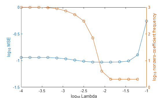
Select the index or indices of Lambda that balance minimal classification error and predictor-variable sparsity (for example, Lambda(11)).

idx = 11;
MdlFinal = selectModels(Mdl,idx);

MdlFinal is a trained RegressionLinear model object that uses Lambda(11) as a regularization strength.

Extended Capabilities

Version History

Introduced in R2016a

expand all