Main Content

binScatterPlot

Scatter plot of bins for tall arrays

Description

example

binScatterPlot(X,Y) creates a binned scatter plot of the data in X and Y. The binScatterPlot function uses an automatic binning algorithm that returns bins with a uniform area, chosen to cover the range of elements in X and Y and reveal the underlying shape of the distribution.

example

binScatterPlot(X,Y,nbins) specifies the number of bins to use in each dimension.

example

binScatterPlot(X,Y,Xedges,Yedges) specifies the edges of the bins in each dimension using the vectors Xedges and Yedges.

example

binScatterPlot(X,Y,Name,Value) specifies additional options with one or more name-value pair arguments using any of the previous syntaxes. For example, you can specify 'Color' and a valid color option to change the color theme of the plot, or 'Gamma' with a positive scalar to adjust the level of detail.

h = binScatterPlot(___) returns a Histogram2 object. Use this object to inspect properties of the plot.

Examples

collapse all

Create two tall vectors of random data. Create a binned scatter plot for the data.

When you perform calculations on tall arrays, MATLAB® uses either a parallel pool (default if you have Parallel Computing Toolbox™) or the local MATLAB session. To run the example using the local MATLAB session when you have Parallel Computing Toolbox, change the global execution environment by using the mapreducer function.

mapreducer(0)

X = tall(randn(1e5,1));
Y = tall(randn(1e5,1));
binScatterPlot(X,Y)
Evaluating tall expression using the Local MATLAB Session:
- Pass 1 of 2: Completed in 0.62 sec
- Pass 2 of 2: Completed in 0.15 sec
Evaluation completed in 1.6 sec
Evaluating tall expression using the Local MATLAB Session:
- Pass 1 of 1: Completed in 0.13 sec
Evaluation completed in 0.18 sec

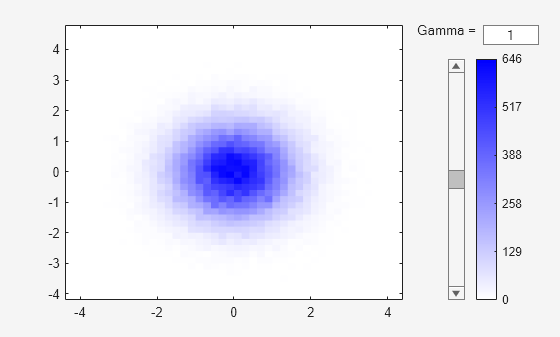
The resulting figure contains a slider to adjust the level of detail in the image.

Specify a scalar value as the third input argument to use the same number of bins in each dimension, or a two-element vector to use a different number of bins in each dimension.

When you perform calculations on tall arrays, MATLAB® uses either a parallel pool (default if you have Parallel Computing Toolbox™) or the local MATLAB session. To run the example using the local MATLAB session when you have Parallel Computing Toolbox, change the global execution environment by using the mapreducer function.

mapreducer(0)

Plot a binned scatter plot of random data sorted into 100 bins in each dimension.

X = tall(randn(1e5,1));
Y = tall(randn(1e5,1));
binScatterPlot(X,Y,100)
Evaluating tall expression using the Local MATLAB Session:
- Pass 1 of 1: Completed in 0.35 sec
Evaluation completed in 0.6 sec
Evaluating tall expression using the Local MATLAB Session:
- Pass 1 of 1: Completed in 0.23 sec
Evaluation completed in 0.43 sec

Use 20 bins in the x-dimension and continue to use 100 bins in the y-dimension.

binScatterPlot(X,Y,[20 100])
Evaluating tall expression using the Local MATLAB Session:
- Pass 1 of 1: Completed in 0.084 sec
Evaluation completed in 0.2 sec
Evaluating tall expression using the Local MATLAB Session:
- Pass 1 of 1: Completed in 0.13 sec
Evaluation completed in 0.19 sec

Plot a binned scatter plot of random data with specific bin edges. Use bin edges of Inf and -Inf to capture outliers.

When you perform calculations on tall arrays, MATLAB® uses either a parallel pool (default if you have Parallel Computing Toolbox™) or the local MATLAB session. To run the example using the local MATLAB session when you have Parallel Computing Toolbox, change the global execution environment by using the mapreducer function.

mapreducer(0)

Create a binned scatter plot with 100 bin edges between [-2 2] in each dimension. The data outside the specified bin edges is not included in the plot.

X = tall(randn(1e5,1));
Y = tall(randn(1e5,1));
Xedges = linspace(-2,2);
Yedges = linspace(-2,2);
binScatterPlot(X,Y,Xedges,Yedges)
Evaluating tall expression using the Local MATLAB Session:
- Pass 1 of 1: Completed in 0.57 sec
Evaluation completed in 0.77 sec

Use coarse bins extending to infinity on the edges of the plot to capture outliers.

Xedges = [-Inf linspace(-2,2) Inf];
Yedges = [-Inf linspace(-2,2) Inf];
binScatterPlot(X,Y,Xedges,Yedges)
Evaluating tall expression using the Local MATLAB Session:
- Pass 1 of 1: Completed in 0.27 sec
Evaluation completed in 0.4 sec

Plot a binned scatter plot of random data, specifying 'Color' as 'c'.

When you perform calculations on tall arrays, MATLAB® uses either a parallel pool (default if you have Parallel Computing Toolbox™) or the local MATLAB session. To run the example using the local MATLAB session when you have Parallel Computing Toolbox, change the global execution environment by using the mapreducer function.

mapreducer(0)

X = tall(randn(1e5,1));
Y = tall(randn(1e5,1));
binScatterPlot(X,Y,'Color','c')
Evaluating tall expression using the Local MATLAB Session:
- Pass 1 of 2: Completed in 0.54 sec
- Pass 2 of 2: Completed in 0.16 sec
Evaluation completed in 1.5 sec
Evaluating tall expression using the Local MATLAB Session:
- Pass 1 of 1: Completed in 0.091 sec
Evaluation completed in 0.13 sec

Input Arguments

collapse all

Data to distribute among bins, specified as separate arguments of tall vectors, matrices, or multidimensional arrays. X and Y must be the same size. If X and Y are not vectors, then binScatterPlot treats them as single column vectors, X(:) and Y(:).

Corresponding elements in X and Y specify the x and y coordinates of 2-D data points, [X(k),Y(k)]. The underlying data types of X and Y can be different, but binScatterPlot concatenates these inputs into a single N-by-2 tall matrix of the dominant underlying data type.

binScatterPlot ignores all NaN values. Similarly, binScatterPlot ignores Inf and -Inf values, unless the bin edges explicitly specify Inf or -Inf as a bin edge.

Note

If X or Y contain integers of type int64 or uint64 that are larger than flintmax, then it is recommended that you explicitly specify the bin edges.binScatterPlot automatically bins the input data using double precision, which lacks integer precision for numbers greater than flintmax.

Data Types: single | double | int8 | int16 | int32 | int64 | uint8 | uint16 | uint32 | uint64 | logical

Number of bins in each dimension, specified as a positive scalar integer or two-element vector of positive integers. If you do not specify nbins, then binScatterPlot automatically calculates how many bins to use based on the values in X and Y.

  • If nbins is a scalar, then binScatterPlot uses that many bins in each dimension.

  • If nbins is a vector, then nbins(1) specifies the number of bins in the x-dimension and nbins(2) specifies the number of bins in the y-dimension.

Example: binScatterPlot(X,Y,20) uses 20 bins in each dimension.

Example: binScatterPlot(X,Y,[10 20]) uses 10 bins in the x-dimension and 20 bins in the y-dimension.

Bin edges in x-dimension, specified as a vector. Xedges(1) is the first edge of the first bin in the x-dimension, and Xedges(end) is the outer edge of the last bin.

The value [X(k),Y(k)] is in the (i,j)th bin if Xedges(i)X(k) < Xedges(i+1) and Yedges(j)Y(k) < Yedges(j+1). The last bins in each dimension also include the last (outer) edge. For example, [X(k),Y(k)] falls into the ith bin in the last row if Xedges(end-1)X(k)Xedges(end) and Yedges(i)Y(k) < Yedges(i+1).

Data Types: single | double | int8 | int16 | int32 | int64 | uint8 | uint16 | uint32 | uint64 | logical

Bin edges in y-dimension, specified as a vector. Yedges(1) is the first edge of the first bin in the y-dimension, and Yedges(end) is the outer edge of the last bin.

The value [X(k),Y(k)] is in the (i,j)th bin if Xedges(i)X(k) < Xedges(i+1) and Yedges(j)Y(k) < Yedges(j+1). The last bins in each dimension also include the last (outer) edge. For example, [X(k),Y(k)] falls into the ith bin in the last row if Xedges(end-1)X(k)Xedges(end) and Yedges(i)Y(k) < Yedges(i+1).

Data Types: single | double | int8 | int16 | int32 | int64 | uint8 | uint16 | uint32 | uint64 | logical

Name-Value Arguments

Specify optional pairs of arguments as Name1=Value1,...,NameN=ValueN, where Name is the argument name and Value is the corresponding value. Name-value arguments must appear after other arguments, but the order of the pairs does not matter.

Before R2021a, use commas to separate each name and value, and enclose Name in quotes.

Example: binScatterPlot(X,Y,'BinWidth',[5 10])

Binning algorithm, specified as the comma-separated pair consisting of 'BinMethod' and one of these values.

ValueDescription
'auto'The default 'auto' algorithm uses a maximum of 100 bins and chooses a bin width to cover the data range and reveal the shape of the underlying distribution.
'scott'Scott’s rule is optimal if the data is close to being jointly normally distributed. This rule is appropriate for most other distributions, as well. It uses a bin size of [3.5*std(X)*numel(X)^(-1/4), 3.5*std(Y)*numel(Y)^(-1/4)].
'integers'The integer rule is useful with integer data, as it creates a bin for each integer. It uses a bin width of 1 and places bin edges halfway between integers. To avoid accidentally creating too many bins, you can use this rule to create a limit of 65536 bins (216). If the data range is greater than 65536, then the integer rule uses wider bins instead.

Note

The BinMethod property of the resulting Histogram2 object always has a value of 'manual'.

Width of bins in each dimension, specified as the comma-separated pair consisting of 'BinWidth' and a scalar or two-element vector of positive integers, [xWidth yWidth]. A scalar value indicates the same bin width for each dimension.

If you specify BinWidth, then binScatterPlot can use a maximum of 1024 bins (210) along each dimension. If instead the specified bin width requires more bins, then binScatterPlot uses a larger bin width corresponding to the maximum number of bins.

Example: binScatterPlot(X,Y,'BinWidth',[5 10]) uses bins with size 5 in the x-dimension and size 10 in the y-dimension.

Plot color theme, specified as the comma-separated pair consisting of 'Color' and one of these options.

OptionDescription
'b'

Blue

'm'

Magenta

'c'

Cyan

'r'

Red

'g'

Green

'y'

Yellow

'k'

Black

Gamma correction, specified as the comma-separated pair consisting of 'Gamma' and a positive scalar. Use this option to adjust the brightness and color intensity to affect the amount of detail in the image.

  • gamma < 1 — As gamma decreases, the shading of bins with smaller bin counts becomes progressively darker, including more detail in the image.

  • gamma > 1 — As gamma increases, the shading of bins with smaller bin counts becomes progressively lighter, removing detail from the image.

  • The default value of 1 does not apply any correction to the display.

Bin limits in x-dimension, specified as the comma-separated pair consisting of 'XBinLimits' and a two-element vector, [xbmin,xbmax]. The vector indicates the first and last bin edges in the x-dimension.

binScatterPlot only plots data that falls within the bin limits inclusively, Data(Data(:,1)>=xbmin & Data(:,1)<=xbmax).

Bin limits in y-dimension, specified as the comma-separated pair consisting of 'YBinLimits' and a two-element vector, [ybmin,ybmax]. The vector indicates the first and last bin edges in the y-dimension.

binScatterPlot only plots data that falls within the bin limits inclusively, Data(Data(:,2)>=ybmin & Data(:,2)<=ybmax).

Output Arguments

collapse all

Binned scatter plot, returned as a Histogram2 object. For more information, see Histogram2 Properties.

Extended Capabilities

Version History

Introduced in R2016b