Main Content

modwtxcorr

Wavelet cross-correlation sequence estimates using the maximal overlap discrete wavelet transform (MODWT)

Description

xcseq = modwtxcorr(w1,w2) returns the wavelet cross-correlation sequence estimates for the maximal overlap discrete wavelet transform (MODWT) transforms specified in w1 and w2. xcseq is a cell array of vectors where the elements in each cell correspond to cross-correlation sequence estimates. If there are enough nonboundary coefficients at the final level, modwtxcorr returns the scaling cross-correlation sequence estimate in the final cell of xcseq.

example

xcseq = modwtxcorr(w1,w2,wav) uses the wavelet wav to determine the number of boundary coefficients by level.

example

[xcseq,xcseqci] = modwtxcorr(___) returns in xcseqci the 95% confidence intervals for the cross-correlation sequence estimates in xcseq, using any arguments from the previous syntaxes.

example

[xcseq,xcseqci] = modwtxcorr(w1,w2,wav,conflevel) uses conflevel for the coverage probability of the confidence interval. conflevel is a real scalar strictly greater than 0 and less than 1. If conflevel is unspecified or specified as empty, the coverage probability defaults to 0.95.

example

[xcseq,xcseqci,lags] = modwtxcorr(___) returns the lags for the wavelet cross-correlation sequence estimates in a cell array of column vectors.

example

[___] = modwtxcorr(___,'reflection') reduces the number of wavelet and scaling coefficients at each scale by half before computing the cross-correlation sequences. Specifying the 'reflection' option in modwtxcorr is equivalent to first obtaining the MODWT of w1 w2 with 'periodic' boundary handling and then computing the wavelet cross-correlation sequence estimates. Use this option only when you obtain the MODWT of w1 and w2 using the 'reflection' boundary condition. You must enter the entire character vector 'reflection'. If you added a wavelet named 'reflection' using the wavelet manager, you must rename that wavelet prior to using this option. 'reflection' may be placed in any position in the input argument list after the input transforms w1 w2.

example

Examples

collapse all

Obtain the MODWT of the Southern Oscillation Index and Truk Islands pressure data. The sampling period is one day.

load soi
load truk
wsoi = modwt(soi);
wtruk = modwt(truk);

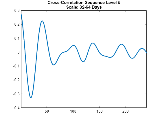
Compute the wavelet cross-correlation sequences. Examine the level-five cross-correlation sequence corresponding to a scale of 32-64 days. Determine the index corresponding to a lag of zero and plot out to 240 lags.

xcseq = modwtxcorr(wsoi,wtruk);
zerolag = floor(numel(xcseq{5})/2)+1;
plot(xcseq{5}(zerolag:zerolag+240),'linewidth',2)
set(gca,'xlim',[1 240]);
title({'Cross-Correlation Sequence Level 5'; 'Scale: 32-64 Days'});
hold off

Figure contains an axes object. The axes object with title Cross-Correlation Sequence Level 5 Scale: 32-64 Days contains an object of type line.

Obtain the MODWT of the Southern Oscillation Index and Truk Islands pressure data using the Fejér-Korovkin wavelet filter with 8 coefficients. The sampling period of the data is one day.

load soi
load truk
wsoi = modwt(soi,'fk8');
wtruk = modwt(truk,'fk8');

Compute the wavelet cross-correlation sequences. Examine the level-five cross-correlation sequence corresponding to a scale of 32-64 days. Determine the index corresponding to a lag of zero and plot out to 240 lags.

xcseq = modwtxcorr(wsoi,wtruk,'fk8');
zerolag = floor(numel(xcseq{5})/2)+1;
plot(xcseq{5}(zerolag:zerolag+240),'linewidth',2)
set(gca,'xlim',[1 240]);
title({'Cross-Correlation Sequence Level 5'; 'Scale: 32-64 Days'});
hold off

Figure contains an axes object. The axes object with title Cross-Correlation Sequence Level 5 Scale: 32-64 Days contains an object of type line.

Plot the wavelet cross-correlation with 95% confidence intervals at scale 4 for two 5-Hz sine wave signals with additive noise.

dt = 0.01;
t = 0:dt:6;
x = cos(2*pi*5*t)+1.5*randn(size(t));
y = cos(2*pi*5*t-pi)+2*randn(size(t));
wx = modwt(x,'fk14',5);
wy = modwt(y,'fk14',5);
modwtcorr(wx,wy,'fk14')
j = 4;
[xcseq,xcseqci] = modwtxcorr(wx,wy,'fk14');
zerolag = floor(numel(xcseq{j})/2)+1;
lagidx = zerolag-30:zerolag+30;
plot(xcseq{j}(lagidx));
hold on;
grid
plot(xcseqci{j}(lagidx,:),'r--');
xlabel('Samples');
title('Scale: 0.32-0.16 Seconds');

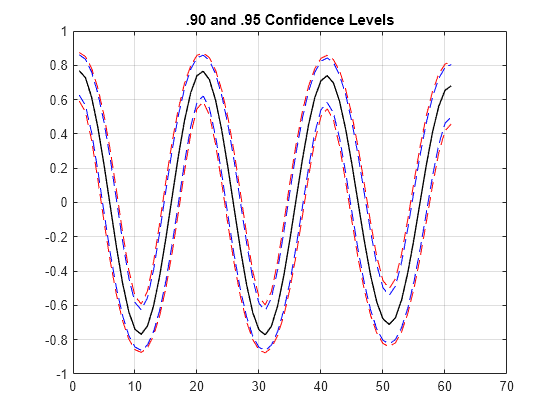
Compare the .90 and .95 (default) confidence intervals for the wavelet cross-correlation at level four.

Obtain the MODWT for two noisy sine waves using the Fejér-Korovkin with 14 coefficients, and specify the level to use.

dt = 0.01;
t = 0:dt:6;
x = cos(2*pi*5*t)+1.5*randn(size(t));
y = cos(2*pi*5*t-pi)+2*randn(size(t));
wx = modwt(x,'fk14',4);
wy = modwt(y,'fk14',4);
lev = 4;

[xcseq,xcseqci] = modwtxcorr(wx,wy,'fk14');
[xcseq90,xcseqci90] = modwtxcorr(wx,wy,'fk14',0.90);
 
zerolag = floor(numel(xcseq{lev})/2)+1;
zerolag90 = floor(numel(xcseq90{lev})/2)+1;
 
lagidx = zerolag-30:zerolag+30;
lagidx90 = zerolag90-30:zerolag90+30;
 
plot(xcseqci{lev}(lagidx,:),'--r');
hold on
plot(xcseqci90{lev}(lagidx90,:),'--b');
plot(xcseq{lev}(lagidx),'-k','LineWidth',1);
grid
title('.90 and .95 Confidence Levels')

Figure contains an axes object. The axes object with title .90 and .95 Confidence Levels contains 5 objects of type line.

Notice that the .95 confidence interval width (in red) is larger than the .90 confidence interval width (in blue).

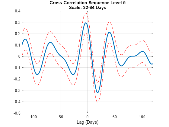
Plot the cross-correlation sequence estimate for the Southern Oscillation Index and Truk Island pressure data. Estimate 95% confidence intervals for scale of 25 days.

load soi
load truk
wsoi = modwt(soi);
wtruk = modwt(truk);
[xcseq,xcseqci,lags] = modwtxcorr(wsoi,wtruk);
plot(lags{5},xcseq{5},'linewidth',2)
hold on
plot(lags{5},xcseqci{5},'r--')
set(gca,'xlim',[-120 120]);
xlabel('Lag (Days)'); 
grid 
title({'Cross-Correlation Sequence Level 5'; 'Scale: 32-64 Days'});
hold off

Figure contains an axes object. The axes object with title Cross-Correlation Sequence Level 5 Scale: 32-64 Days, xlabel Lag (Days) contains 3 objects of type line.

Obtain the MODWT of 36 years of Southern Oscillation Index and Truk Islands pressure data with both periodic and reflection boundary conditions. The modwt function with the 'reflection' option extends the input signal symmetrically at the right boundary. The input signal is then twice its original length. MODWTXCORR with the reflection boundary handling reduces the number of wavelet and scaling coefficients at each half before computing the cross-correlation sequences. The size of the cross-correlation sequences is the same as acquiring the MODWT with the default periodic boundary condition.

load soi
load truk

Obtain the MODWT with the default periodic boundary condition.

wsoi_default = modwt(soi); 
wtruk_default = modwt(truk);

Obtain the MODWT with the reflection boundary condition.

wsoi_reflect = modwt(soi,'reflection');
wtruk_reflect = modwt(truk,'reflection');

Obtain the cross-correlation sequences.

xcseq_default = modwtxcorr(wsoi_default,wtruk_default);
xcseq_reflect = modwtxcorr(wsoi_reflect,wtruk_reflect,'reflection');

Compare the number of elements in the cell array output for both boundary conditions.

cellfun(@numel,xcseq_reflect)
ans = 10×1

       25981
       25953
       25897
       25785
       25561
       25113
       24217
       22425
       18841
       11673

cellfun(@numel,xcseq_default)
ans = 10×1

       25981
       25953
       25897
       25785
       25561
       25113
       24217
       22425
       18841
       11673

Input Arguments

collapse all

MODWT transform of signal 1, specified as a matrix. The input w1 must be the same size as w2 and must have been obtained with the same wavelet. By default, modwtxcorr assumes that you obtained the MODWT using the symlet wavelet with four vanishing moments, 'sym4'.

Data Types: double

MODWT transform of signal 2, specified as a matrix. The input w2 must be the same size as w1 and must have been obtained with the same wavelet. By default, modwtxcorr assumes that you obtained the MODWT using the symlet wavelet with four vanishing moments ('sym4').

Data Types: double

Wavelet, specified as a character vector or string scalar, indicating a valid wavelet, or as a positive even integer indicating the length of the wavelet and scaling filters. If wav is unspecified or specified as an empty, [], wav defaults to 'sym4'.

Data Types: double | char | string

Confidence level, specified as a positive scalar less than 1. conflevel determines the coverage probability of the confidence intervals in xcseqci. If unspecified, or specified as empty, [], conflevel defaults to 0.95.

Data Types: double

Output Arguments

collapse all

Cross-correlation sequences by scale, returned as a cell array of vectors. The vectors are of size 2NJ-by-1, where NJ is the number of nonboundary coefficients by level (scale). This level is the minimum of size(w1,1) and floor(log2(N/(L-1)+1)) where N is the length of the data and L is the filter length. If there are enough nonboundary coefficients at the final level, modwtxcorr returns the scaling cross-correlation sequence estimate in the final cell of xcseq.

Confidence intervals by scale, returned as a cell array of matrices. The size of each matrix is (2NJ-1)-by-2, where NJ is the number of nonboundary coefficients by level (scale).

  • For the .95 default value, the first column of the ith element of xcseqci contains the lower 95% confidence bound for the cross-correlation coefficient at each lag.

  • For the .95 default value, the second column contains the upper 95% confidence bound.

Confidence bounds are computed using Fisher's Z-transformation. The standard error of Fisher's Z statistic is the square root of N–3. In this case, N is the equivalent number of coefficients in the critically sampled discrete wavelet transform (DWT), floor(size(w1,2)/2^LEV), where LEV is the level of the wavelet transform. modwtcorr returns NaNs for the confidence bounds when N-3 is less than or equal to zero.

Lags for the cross-correlation sequences, returned as a cell array of vectors. lags is a cell array of column vectors the same length as xcseq. The elements in each cell of xcseq correspond to the cross-correlation sequence estimates at lags from -(NJ-1) to (NJ-1), where NJ is the number of nonboundary coefficients at level J. The 0th lag element is located at the index floor((2*NJ-1)/2)+1.

References

[1] Percival, D. B., and A. T. Walden. Wavelet Methods for Time Series Analysis. Cambridge, UK: Cambridge University Press, 2000.

[2] Whitcher, B., P. Guttorp, and D. B. Percival. "Wavelet analysis of covariance with application to atmospheric time series." Journal of Geophysical Research, Vol. 105, 2000, pp. 14941–14962.

Version History

Introduced in R2015b

Go to top of page