802.11be System-Level Simulation Using STR Multi-Link Operation

This example shows how to simulate an IEEE® 802.11be™ (Wi-Fi® 7) [1] simultaneous transmit and receive (STR) multi-link operation (MLO) between an access point (AP) multi-link device (MLD) and a station (STA) MLD.

Using this example, you can:

1. Simulate MLO communication between an AP MLD and a STA MLD.

2. Visualize the packet communication in the time and frequency domains for each link of the AP MLD and the STA MLD.

3. Capture the application layer (APP), medium access control layer (MAC), and physical layer (PHY) statistics for each node.

The simulation results show performance metrics such as MAC throughput, MAC packet loss, and application packet latency captured at each node. The results also show how to calculate the throughput and packet loss ratio obtained on each link within an MLD node.

Additionally, you can further explore the example by performing these tasks.

• Impact of Varying Number of Links in MLD on Throughput and Latency

• Faster Execution Using Parallel Simulation Runs

802.11be Multi-Link Operation

The multi-link operation capability introduced in the IEEE 802.11be standard plays an important role in enhancing data rates, reducing latency, and improving reliability. An 802.11be device, whether an access point or a station, qualifies as an MLD if it possesses the capability to facilitate MLO communication across multiple links. These links, within an MLD, operate on different frequencies.

An MLD, when equipped with multiple 802.11be radios, can operate in either the STR mode or the non-simultaneous transmit and receive (NSTR) mode. This operation depends on the ability of the MLD to concurrently transmit and receive packets across different links.

Additionally, a station MLD can support more advanced multi-link operating modes, such as enhanced multi-link single-radio (EMLSR) or enhanced multi-link multi-radio (EMLMR). A station MLD with a single 802.11be radio can operate in EMLSR mode if it can listen for control frames from an AP MLD on one or more links simultaneously, followed by MAC frame exchanges on a single link. Conversely, a station MLD that has multiple 802.11be radios and the ability to dynamically reconfigure spatial multiplexing across multiple links can operate in EMLMR mode.

For more information about MLO, see Overview of Wi-Fi 7 (IEEE 802.11be).

MLO System-Level Simulation Scenario

This example simulates an 802.11be network consisting of an AP MLD and a STA MLD operating in STR mode. The AP MLD and the STA MLD maintain three associated links, operating at frequency bands of 2.4 GHz, 5 GHz, and 6 GHz. This scenario configures bidirectional data traffic, enabling data flow from the AP to the STA and from the STA to the AP. At the end of the simulation, capture the statistics and compute the transmission throughput for the AP and STA.

Configure Simulation Parameters

Set the seed for the random number generator to 1. The seed value controls the pattern of random number generation. The random number generated by the seed value impacts several processes within the simulation, including backoff counter selection at the MAC layer and predicting packet reception success at the physical layer. To improve the accuracy of your simulation results after running the simulation, you can change the seed value, run the simulation again, and average the results over multiple simulations.

rng(1,"combRecursive")

Specify the simulation time in seconds. To visualize the packet communication for all of the nodes, set the enablePacketVisualization variable to true. To view the node performance visualization, set the enableNodePerformancePlot variable to true.

simulationTime = 1;
enablePacketVisualization = true;
enableNodePerformancePlot = true;

Configure WLAN Scenario

Initialize the wireless network simulator.

networkSimulator = wirelessNetworkSimulator.init;

Nodes

Specify the [band channel] pairs for each link in the MLD node.

bandAndChannelValues = [2.4 1; 5 36; 6 1];
numLinks = size(bandAndChannelValues,1);

Create and configure an AP MLD and a STA MLD by using the wlanNode, wlanMultilinkDeviceConfig, and wlanLinkConfig objects.

Create a wlanLinkConfig object for each link of the AP MLD and of the STA MLD, specifying the BandAndChannel, MCS, MPDUAggregationLimit, and TransmitPower property values. Note that both the AP and STA link configuration objects must have the same MPDUAggreggationLimit value.

for linkIdx = 1:numLinks
    apLinkCfg(linkIdx) = wlanLinkConfig(BandAndChannel=bandAndChannelValues(linkIdx,:),MCS=2,MPDUAggregationLimit=100,TransmitPower=15);
    staLinkCfg(linkIdx) = wlanLinkConfig(BandAndChannel=bandAndChannelValues(linkIdx,:),MCS=3,MPDUAggregationLimit=100,TransmitPower=15); %#ok<*SAGROW>
end

Specify the MLD level configuration parameters for the AP MLD and the STA MLD by using the wlanMultilinkDeviceConfig object. Create two separate WLAN multi-link device configuration objects: one for the AP MLD and another for the STA MLD. Configure an MLD as an AP or a STA by setting the Mode property of the wlanMultilinkDeviceConfig object to "AP" or "STA", respectively.

apMLDCfg = wlanMultilinkDeviceConfig(Mode="AP",LinkConfig=apLinkCfg);
apMLD = wlanNode(Position=[0 0 0],Name="AP",DeviceConfig=apMLDCfg);

staMLDCfg = wlanMultilinkDeviceConfig(Mode="STA",LinkConfig=staLinkCfg);
staMLD = wlanNode(Position=[10 0 0],Name="STA",DeviceConfig=staMLDCfg);

nodes = [apMLD staMLD];

To visualize the node positions in the Cartesian plane, use the wirelessNetworkViewer object. Initialize the object with an appropriate canvas size. Add the AP and the STA to the wirelessNetworkViewer object by using the addNodes object function.

networkViewerObj = wirelessNetworkViewer(CanvasSize=[50 50 0]);
addNodes(networkViewerObj,apMLD,Type="AP");
addNodes(networkViewerObj,staMLD,Type="STA");

Association

Associate the STA MLD to the AP MLD by using the associateStations object function of the wlanNode object. To configure uplink and downlink application traffic between the AP and STA, specify the FullBufferTraffic argument of the associateStations object function.

associateStations(apMLD,staMLD,FullBufferTraffic="on")

Wireless Channel

To model a random TGax fading channel between each node, this example uses the hSLSTGaxMultiFrequencySystemChannel helper object. Add the channel model to the wireless network simulator by using the addChannelModel (Wireless Network Toolbox) object function of the wirelessNetworkSimulator object.

channel = hSLSTGaxMultiFrequencySystemChannel(nodes);
addChannelModel(networkSimulator,channelFunction(channel))

Simulation and Results

Add the nodes to the wireless network simulator.

addNodes(networkSimulator,nodes)

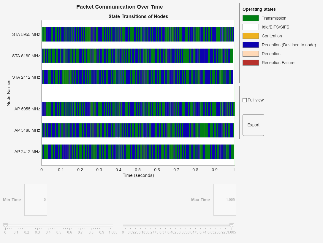
To visualize the packet communication, use the wirelessTrafficViewer object. The visualization shows these plots:

• Packet communication over the time and frequency domains.

• State transitions of each node over time.

Add the nodes to the wirelessTrafficViewer object by using the addNodes object function.

if enablePacketVisualization
    packetVisObj = wirelessTrafficViewer;
    addNodes(packetVisObj,nodes);
end

To view the node performance visualization, use the helperPerformanceViewer helper object.

perfViewerObj = helperPerformanceViewer(nodes,simulationTime);

Run the network simulation for the specified simulation time. The runtime visualization shows the packet communication in the time and frequency domains for the AP and the STA.

run(networkSimulator,simulationTime)

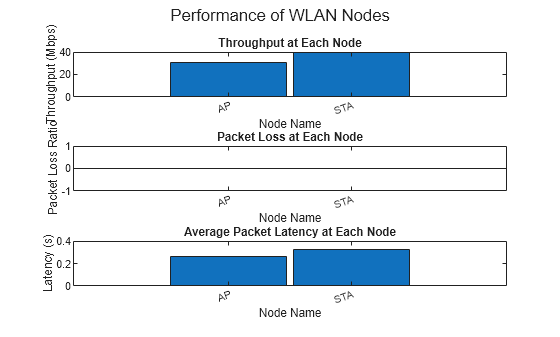
The plotNetworkStats object function displays these simulation plots.

• MAC throughput (in Mbps) at each transmitter (AP MLD and STA MLD).

• MAC packet loss ratio (ratio of unsuccessful data transmissions to the total data transmissions) at each transmitter (AP MLD and STA MLD).

• Average application packet latency (in seconds) incurred at each receiver (AP MLD and STA MLD). The average application packet latency shows the average latency that the STA MLD incurs to receive the downlink traffic from the AP MLD and the average latency that the AP MLD incurs to receive uplink traffic from the STA MLD.

if enableNodePerformancePlot
    plotNetworkStats(perfViewerObj)
end

Statistics for Each Link in MLD

Retrieve the APP, MAC, and PHY statistics at each node by using the statistics object function of the wlanNode object. You can also access the statistics for each link of the MLD node from within the MAC and PHY substructures of the statistics structure. To retrieve the statistics for each link, specify the "all" argument to the statistics object function.

stats = statistics(nodes,"all");

The Link substructure within the MAC and PHY layer statistics structures contains the link-level statistics of the MLD node. For more information about the statistics, see WLAN System-Level Simulation Statistics.

stats(1).MAC.Link

ans=1×3 struct array with fields:
    TransmittedDataFrames
    TransmittedPayloadBytes
    SuccessfulDataTransmissions
    RetransmittedDataFrames
    TransmittedAMPDUs
    TransmittedRTSFrames
    TransmittedMURTSFrames
    TransmittedCTSFrames
    TransmittedMUBARFrames
    TransmittedAckFrames
    TransmittedBlockAckFrames
    TransmittedCFEndFrames
    TransmittedBasicTriggerFrames
    TransmittedBeaconFrames
    ReceivedDataFrames
    ReceivedPayloadBytes
    ReceivedAMPDUs
    ReceivedRTSFrames
    ReceivedMURTSFrames
    ReceivedCTSFrames
    ReceivedMUBARFrames
    ReceivedAckFrames
    ReceivedBlockAckFrames
    ReceivedCFEndFrames
    ReceivedBasicTriggerFrames
    ReceivedFCSValidFrames
    ReceivedFCSFails
    ReceivedDelimiterCRCFails
    ReceivedBeaconFrames
    AccessCategories
      ⋮

Calculate the MAC throughput (in Mbps) at the MLD node and at each link in the MLD node by using the throughput object function of helperPerformanceViewer helper object.

apMLDThroughput = throughput(perfViewerObj,apMLD.ID)

apMLDThroughput = 
29.2680

apLink1Throughput = throughput(perfViewerObj,apMLD.ID,LinkID=1)

apLink1Throughput = 
10.3680

apLink2Throughput = throughput(perfViewerObj,apMLD.ID,LinkID=2)

apLink2Throughput = 
9.8280

apLink3Throughput = throughput(perfViewerObj,apMLD.ID,LinkID=3)

apLink3Throughput = 
9.0720

Calculate the MAC packet loss ratio at the MLD node and at each link in the MLD node by using the packetLossRatio object function of helperPerformanceViewer helper object.

apMLDPLR = packetLossRatio(perfViewerObj,apMLD.ID)

apMLDPLR = 
0

apLink1PLR = packetLossRatio(perfViewerObj,apMLD.ID,LinkID=1)

apLink1PLR = 
0

apLink2PLR = packetLossRatio(perfViewerObj,apMLD.ID,LinkID=2)

apLink2PLR = 
0

apLink3PLR = packetLossRatio(perfViewerObj,apMLD.ID,LinkID=3)

apLink3PLR = 
0

Further Exploration

You can use this example to further explore these functionalities.

Impact of Variable Number of Links in MLD on Throughput and Latency

Generate MAC throughput and application latency results for scenarios consisting of an AP MLD and two associated STA MLDs by using the hSimulateMLOWithVaryingLinks helper function. Using this helper function, you can perform these tasks.

• Simulate scenarios with variable number of links and application traffic data rates.

• Plot the throughput and latency results as a function of the application traffic data rates.

By default, this helper function plots the stored throughput and latency values. To reproduce these results, set the plotStoredThroughputValues value to false.

plotStoredThroughputValues = true;
hSimulateMLOWithVaryingLinks(plotStoredThroughputValues)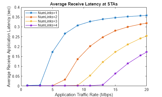

These plots compare throughput and latency by considering a variable number of links in the MLD. Due to an increase in simultaneous transmissions, the AP MLD achieves higher throughput under significant traffic loads and with more available links. Likewise, as you increase the number of links between the AP MLD and STA MLD, the average latency that the receiving stations experience decreases. This decrease in latency becomes more noticeable with an increase in traffic load.

Faster Execution Using Parallel Simulation Runs

If you want to run multiple simulations, you can speed up the simulations by enabling parallel computing using the parfor loop. The parfor loop is an alternative to the for loop that enables you to execute multiple simulation runs in parallel, thereby reducing total execution time. To use parfor, you must have a Parallel Computing Toolbox™ license. For more information about running multiple simulations by using a parfor loop, see the hSimulateMLOWithVaryingLinks helper function.

Appendix

The example uses these helpers:

• hSLSTGaxMultiFrequencySystemChannel — Return a system channel object, and set the path loss model

• hSLSTGaxAbstractSystemChannel — Return a channel object for the abstracted PHY layer

• hSLSTGaxSystemChannel — Return a channel object for the full PHY layer

• hSLSTGaxSystemChannelBase — Return the base channel object

• hSimulateMLOWithVaryingLinks — Simulate and plot throughput and latency for variable number of links

• helperPerformanceViewer — Return a performance metrics viewer object

References

1. “IEEE Standard for Information Technology–Telecommunications and Information Exchange between Systems Local and Metropolitan Area Networks–Specific Requirements - Part 11: Wireless LAN Medium Access Control (MAC) and Physical Layer (PHY) Specifications Amendment 2: Enhancements for Extremely High Throughput (EHT).” IEEE Std 802.11be-2024 (Amendment to IEEE Std 802.11-2024, as Amended by 802.11bh-2024), July 2025, 1–1020. https://doi.org/10.1109/IEEESTD.2024.11090080.