Results for
In a recent blog post, @Guy Rouleau writes about the new Simulink Copilot Beta. Sign ups are on the Copilot Beta page below. Let him know what you think.
Guy's Blog Post - https://blogs.mathworks.com/simulink/2025/12/01/a-copilot-for-simulink/
Simulink Copilot Beta - https://www.mathworks.com/products/simulink-copilot.html
If you haven't solved the problem yet, below hints guide how the algorithm should be implemented and clarify subtle rules that are easy to miss.
1. Shield is ONLY defended in HOME matches of the CURRENT holder - Even if a team beats the Shield holder in an away match, that does NOT count as a Shield defense.
2. A team defends the Shield ONLY when:
> They currently hold it.
> They are home team in that match
3. Shield transfer happens ONLY if the HOLDER plays a home match AND loses - A team may lose an away match — no effect.
4. The output ALWAYS includes the initial holder as the first row.
5. Defenses count resets for each new holder. - Every holder accumulates their own count until they lose it at home.
6. Match numbers are 1-indexed in the input, but “0” is used for initial state - The first real match is Match 1, but the output starts with Match 0.
7. Output row is created ONLY WHEN SHIELD CHANGES HANDS - This is an important hidden detail. A new row is appended, When the current holder loses a home match → Shield taken by visitor. If no loss at home occurs after that → no new row until next change.
8. The last holder’s defense count goes until the season ends - Even if they lose away later.
9. If a holder never gets a home match, defenses = 0.
10. In case the holder loses their very first home match → defenses = 0.
11. Shield changes only on HOME LOSS, not on a draw.
I hope above hints will help you in solving the problem.
Thanks and Regards,
Dev

% Recreation of Saturn photo
figure('Color', 'k', 'Position', [100, 100, 800, 800]);
ax = axes('Color', 'k', 'XColor', 'none', 'YColor', 'none', 'ZColor', 'none');
hold on;
% Create the planet sphere
[x, y, z] = sphere(150);
% Saturn colors - pale yellow/cream gradient
saturn_radius = 1;
% Create color data based on latitude for gradient effect
lat = asin(z);
color_data = rescale(lat, 0.3, 0.9);
% Plot Saturn with smooth shading
planet = surf(x*saturn_radius, y*saturn_radius, z*saturn_radius, ...
color_data, ...
'EdgeColor', 'none', ...
'FaceColor', 'interp', ...
'FaceLighting', 'gouraud', ...
'AmbientStrength', 0.3, ...
'DiffuseStrength', 0.6, ...
'SpecularStrength', 0.1);
% Use a cream/pale yellow colormap for Saturn
cream_map = [linspace(0.4, 0.95, 256)', ...
linspace(0.35, 0.9, 256)', ...
linspace(0.2, 0.7, 256)'];
colormap(cream_map);
% Create the ring system
n_points = 300;
theta = linspace(0, 2*pi, n_points);
% Define ring structure (inner radius, outer radius, brightness)
rings = [
1.2, 1.4, 0.7; % Inner ring
1.45, 1.65, 0.8; % A ring
1.7, 1.85, 0.5; % Cassini division (darker)
1.9, 2.3, 0.9; % B ring (brightest)
2.35, 2.5, 0.6; % C ring
2.55, 2.8, 0.4; % Outer rings (fainter)
];
% Create rings as patches
for i = 1:size(rings, 1)
r_inner = rings(i, 1);
r_outer = rings(i, 2);
brightness = rings(i, 3);
% Create ring coordinates
x_inner = r_inner * cos(theta);
y_inner = r_inner * sin(theta);
x_outer = r_outer * cos(theta);
y_outer = r_outer * sin(theta);
% Front side of rings
ring_x = [x_inner, fliplr(x_outer)];
ring_y = [y_inner, fliplr(y_outer)];
ring_z = zeros(size(ring_x));
% Color based on brightness
ring_color = brightness * [0.9, 0.85, 0.7];
fill3(ring_x, ring_y, ring_z, ring_color, ...
'EdgeColor', 'none', ...
'FaceAlpha', 0.7, ...
'FaceLighting', 'gouraud', ...
'AmbientStrength', 0.5);
end
% Add some texture/gaps in the rings using scatter
n_particles = 3000;
r_particles = 1.2 + rand(1, n_particles) * 1.6;
theta_particles = rand(1, n_particles) * 2 * pi;
x_particles = r_particles .* cos(theta_particles);
y_particles = r_particles .* sin(theta_particles);
z_particles = (rand(1, n_particles) - 0.5) * 0.02;
% Vary particle brightness
particle_colors = repmat([0.8, 0.75, 0.6], n_particles, 1) .* ...
(0.5 + 0.5*rand(n_particles, 1));
scatter3(x_particles, y_particles, z_particles, 1, particle_colors, ...
'filled', 'MarkerFaceAlpha', 0.3);
% Add dramatic outer halo effect - multiple layers extending far out
n_glow = 20;
for i = 1:n_glow
glow_radius = 1 + i*0.35; % Extend much farther
alpha_val = 0.08 / sqrt(i); % More visible, slower falloff
% Color gradient from cream to blue/purple at outer edges
if i <= 8
glow_color = [0.9, 0.85, 0.7]; % Warm cream/yellow
else
% Gradually shift to cooler colors
mix = (i - 8) / (n_glow - 8);
glow_color = (1-mix)*[0.9, 0.85, 0.7] + mix*[0.6, 0.65, 0.85];
end
surf(x*glow_radius, y*glow_radius, z*glow_radius, ...
ones(size(x)), ...
'EdgeColor', 'none', ...
'FaceColor', glow_color, ...
'FaceAlpha', alpha_val, ...
'FaceLighting', 'none');
end
% Add extensive glow to rings - make it much more dramatic
n_ring_glow = 12;
for i = 1:n_ring_glow
glow_scale = 1 + i*0.15; % Extend farther
alpha_ring = 0.12 / sqrt(i); % More visible
for j = 1:size(rings, 1)
r_inner = rings(j, 1) * glow_scale;
r_outer = rings(j, 2) * glow_scale;
brightness = rings(j, 3) * 0.5 / sqrt(i);
x_inner = r_inner * cos(theta);
y_inner = r_inner * sin(theta);
x_outer = r_outer * cos(theta);
y_outer = r_outer * sin(theta);
ring_x = [x_inner, fliplr(x_outer)];
ring_y = [y_inner, fliplr(y_outer)];
ring_z = zeros(size(ring_x));
% Color gradient for ring glow
if i <= 6
ring_color = brightness * [0.9, 0.85, 0.7];
else
mix = (i - 6) / (n_ring_glow - 6);
ring_color = brightness * ((1-mix)*[0.9, 0.85, 0.7] + mix*[0.65, 0.7, 0.9]);
end
fill3(ring_x, ring_y, ring_z, ring_color, ...
'EdgeColor', 'none', ...
'FaceAlpha', alpha_ring, ...
'FaceLighting', 'none');
end
end
% Add diffuse glow particles for atmospheric effect
n_glow_particles = 8000;
glow_radius_particles = 1.5 + rand(1, n_glow_particles) * 5;
theta_glow = rand(1, n_glow_particles) * 2 * pi;
phi_glow = acos(2*rand(1, n_glow_particles) - 1);
x_glow = glow_radius_particles .* sin(phi_glow) .* cos(theta_glow);
y_glow = glow_radius_particles .* sin(phi_glow) .* sin(theta_glow);
z_glow = glow_radius_particles .* cos(phi_glow);
% Color particles based on distance - cooler colors farther out
particle_glow_colors = zeros(n_glow_particles, 3);
for i = 1:n_glow_particles
dist = glow_radius_particles(i);
if dist < 3
particle_glow_colors(i,:) = [0.9, 0.85, 0.7];
else
mix = (dist - 3) / 4;
particle_glow_colors(i,:) = (1-mix)*[0.9, 0.85, 0.7] + mix*[0.5, 0.6, 0.9];
end
end
scatter3(x_glow, y_glow, z_glow, rand(1, n_glow_particles)*2+0.5, ...
particle_glow_colors, 'filled', 'MarkerFaceAlpha', 0.05);
% Lighting setup
light('Position', [-3, -2, 4], 'Style', 'infinite', ...
'Color', [1, 1, 0.95]);
light('Position', [2, 3, 2], 'Style', 'infinite', ...
'Color', [0.3, 0.3, 0.4]);
% Camera and view settings
axis equal off;
view([-35, 25]); % Angle to match saturn_photo.jpg - more dramatic tilt
camva(10); % Field of view - slightly wider to show full halo
xlim([-8, 8]); % Expanded to show outer halo
ylim([-8, 8]);
zlim([-8, 8]);
% Material properties
material dull;
title('Saturn - Left click: Rotate | Right click: Pan | Scroll: Zoom', 'Color', 'w', 'FontSize', 12);
% Enable interactive camera controls
cameratoolbar('Show');
cameratoolbar('SetMode', 'orbit'); % Start in rotation mode

% Custom mouse controls
set(gcf, 'WindowButtonDownFcn', @mouseDown);
function mouseDown(src, ~)
selType = get(src, 'SelectionType');
switch selType
case 'normal' % Left click - rotate
cameratoolbar('SetMode', 'orbit');
rotate3d on;
case 'alt' % Right click - pan
cameratoolbar('SetMode', 'pan');
pan on;
end
end
Many MATLAB Cody problems involve solving congruences, modular inverses, Diophantine equations, or simplifying ratios under constraints. A powerful tool for these tasks is the Extended Euclidean Algorithm (EEA), which not only computes the greatest common divisor, gcd(a,b), but also provides integers x and y such that: a*x + b*y = gcd(a,b) - which is Bezout's identity.
Use of the Extended Euclidean Algorithm is very using in solving many different types of MATLAB Cody problems such as:
- Computing modular inverses safely, even for very large numbers
- Solving linear Diophantine equations
- Simplifing fractions or finding nteger coefficients without using symbolic tools
- Avoiding loops (EEA can be implemented recursively)
Below is a recursive implementation of the EEA.
function [g,x,y] = egcd(a,b)
% a*x + b*y = g [gcd(a,b)]
if b == 0
g = a; x = 1; y = 0;
else
[g, x1, y1] = egcd(b, mod(a,b));
x = y1;
y = x1 - floor(a/b)*y1;
end
end
Problem:
Given integers a and m, return the modular inverse of a (mod m).
If the inverse does not exist, return -1.
function inv = modInverse(a,m)
[g,x,~] = egcd(a,m);
if g ~= 1 % inverse doesn't exist
inv = -1;
else
inv = mod(x,m); % Bézout coefficient gives the inverse
end
end
%find the modular inverse of 19 (mod 5)
inv=modInverse(19,5)
Congratulations to all the Relentless Coders who have completed the problem set. I hope you weren't too busy relentlessly solving problems to enjoy the silliness I put into them.
If you've solved the whole problem set, don't forget to help out your teammates with suggestions, tips, tricks, etc. But also, just for fun, I'm curious to see which of my many in-jokes and nerdy references you noticed. Many of the problems were inspired by things in the real world, then ported over into the chaotic fantasy world of Nedland.
I guess I'll start with the obvious real-world reference: @Ned Gulley (I make no comment about his role as insane despot in any universe, real or otherwise.)
Hi Everyone!
As this is the most difficult question in problem group "Cody Contest 2025". To solve this problem, It is very important to understand all the hidden clues in the problem statement. Because everything is not directly visible.
For those who tried the problem, but were not able to solve. You might have missed any of the below hints -
- “The other players do not get to see which card has been shown, but they do know which three cards were asked for and that the player asked had one of them.” - Even when the card identity isn’t revealed (result = 0), you still gain partial knowledge — the asked player must have at least one of those three cards, meaning you can mark other players as not having all three simultaneously.
- "If it is your turn, you know the exact identity of that card" - You only know the exact shown card when result = 1, 2, or 3 — and it must be your turn. If someone else asked (even if you know result = 0), you don’t know which one was shown. So the meaning of result depends on whose turn it was, which is implicit — MATLAB code must assume that turns alternate 1→m→1, so your turn index is determined by (t-1) mod m + 1 == pnum.
- "Any leftover cards are placed face-up so that all players can see them" - These cards (commoncards) are not in anyone’s hand and cannot be in the envelope. So they’re not just visible — they’re logical constraints to eliminate from deduction.
- “It may be possible to determine the solution from less information than is given, but the information given will always be sufficient.”
- "Turn order is implied, not given explicitly" - Players take turns in order (1 to m, and back to 1).
On considering all the clues and constraints in the question, you will definitely be able to card for each category present in envelope.
I hope above clues will be useful for you.
Thank you, wishing you the success!
Regards,
Dev
Experimenting with Agentic AI
44%
I am an AI skeptic
0%
AI is banned at work
11%
I am happy with Conversational AI
44%
9 votes
When solving Cody problems, sometimes your solution takes too long — especially if you’re recomputing large arrays or iterative sequences every time your function is called.
The Cody work area resets between separate runs of your code, but within one Cody test suite, your function may be called multiple times in a single session.
This is where persistent variables come in handy.
A persistent variable keeps its value between function calls, but only while MATLAB is still running your function suite.
This means:
- You can cache results to avoid recomputation.
- You can accumulate data across multiple calls.
- But it resets when Cody or MATLAB restarts.
Suppose you’re asked to find the n-th Fibonacci number efficiently — Cody may time out if you use recursion naively. Here’s how to use persistent to store computed values:
function f = fibPersistent(n)
import java.math.BigInteger
persistent F
if isempty(F)
F=[BigInteger('0'),BigInteger('1')];
for k=3:10000
F(k)=F(k-1).add(F(k-2));
end
end
% Extend the stored sequence only if needed
while length(F) <= n
F(end+1)=F(end).add(F(end-1));
end
f = char(F(n+1).toString); % since F(1) is really F(0)
end
%calling function 100 times
K=arrayfun(@(x)fibPersistent(x),randi(10000,1,100),'UniformOutput',false);
K(100)
The fzero function can handle extremely messy equations — even those mixing exponentials, trigonometric, and logarithmic terms — provided the function is continuous near the root and you give a reasonable starting point or interval.
It’s ideal for cases like:
- Solving energy balance equations
- Finding intersection points of nonlinear models
- Determining parameters from experimental data
Example: Solving for Equilibrium Temperature in a Heat Radiation-Conduction Model
Suppose a spacecraft component exchanges heat via conduction and radiation with its environment. At steady state, the power generated internally equals the heat lost:
Given constants:
 = 25 W
- k = 0.5 W/K
- ϵ = 0.8
- σ = 5.67e−8 W/m²K⁴
- A = 0.1 m²
 = 250 K
Find the steady-state temperature, T.
% Given constants
Qgen = 25;
k = 0.5;
eps = 0.8;
sigma = 5.67e-8;
A = 0.1;
Tinf = 250;
% Define the energy balance equation (set equal to zero)
f = @(T) Qgen - (k*(T - Tinf) + eps*sigma*A*(T.^4 - Tinf^4));
% Plot for a sense of where the root lies before implementing
fplot(f, [250 300]); grid on
xlabel('Temperature (K)'); ylabel('f(T)')
title('Energy Balance: Root corresponds to steady-state temperature')
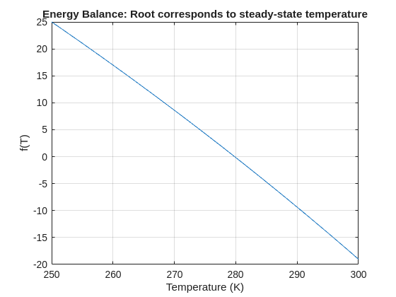
% Use fzero with an interval that brackets the root
T_eq = fzero(f, [250 300]);
fprintf('Steady-state temperature: %.2f K\n', T_eq);
I set my 3D matrix up with the players in the 3rd dimension. I set up the matrix with: 1) player does not hold the card (-1), player holds the card (1), and unknown holding the card (0). I moved through the turns (-1 and 1) that are fixed first. Then cycled through the conditional turns (0) while checking the cards of each player using the hints provided until it was solved. The key for me in solving several of the tests (11, 17, and 19) was looking at the 1's and 0's being held by each player.
sum(cardState==1,3);%any zeros in this 2D matrix indicate possible cards in the solution
sum(cardState==0,3)>0;%the ones in this 2D matrix indicate the only unknown positions
sum(cardState==1,3)|sum(cardState==0,3)>0;%oring the two together could provide valuable information
Some MATLAB Cody problems prohibit loops (for, while) or conditionals (if, switch, while), forcing creative solutions.
One elegant trick is to use nested functions and recursion to achieve the same logic — while staying within the rules.
Example: Recursive Summation Without Loops or Conditionals
Suppose loops and conditionals are banned, but you need to compute the sum of numbers from 1 to n. This is a simple example and obvisously n*(n+1)/2 would be preferred.
function s = sumRecursive(n)
zero=@(x)0;
s = helper(n); % call nested recursive function
function out = helper(k)
L={zero,@helper};
out = k+L{(k>0)+1}(k-1);
end
end
sumRecursive(10)
- The helper function calls itself until the base case is reached.
- Logical indexing into a cell array (k>0) act as an 'if' replacement.
- MATLAB allows nested functions to share variables and functions (zero), so you can keep state across calls.
Tips:
- Replace 'if' with logical indexing into a cell array.
- Replace for/while with recursion.
- Nested functions are local and can access outer variables, avoiding global state.
Many MATLAB Cody problems involve recognizing integer sequences.
If a sequence looks familiar but you can’t quite place it, the On-Line Encyclopedia of Integer Sequences (OEIS) can be your best friend.
OEIS will often identify the sequence, provide a formula, recurrence relation, or even direct MATLAB-compatible pseudocode.
Example: Recognizing a Cody Sequence
Suppose you encounter this sequence in a Cody problem:
1, 1, 2, 3, 5, 8, 13, 21, ...
Entering it on OEIS yields A000045 – The Fibonacci Numbers, defined by:
F(n) = F(n-1) + F(n-2), with F(1)=1, F(2)=1
You can then directly implement it in MATLAB:
function F = fibSeq(n)
F = zeros(1,n);
F(1:2) = 1;
for k = 3:n
F(k) = F(k-1) + F(k-2);
end
end
fibSeq(15)
When solving MATLAB Cody problems involving very large integers (e.g., factorials, Fibonacci numbers, or modular arithmetic), you might exceed MATLAB’s built-in numeric limits.
To overcome this, you can use Java’s java.math.BigInteger directly within MATLAB — it’s fast, exact, and often accepted by Cody if you convert the final result to a numeric or string form.
Below is an example of using it to find large factorials.
function s = bigFactorial(n)
import java.math.BigInteger
f = BigInteger('1');
for k = 2:n
f = f.multiply(BigInteger(num2str(k)));
end
s = char(f.toString); % Return as string to avoid overflow
end
bigFactorial(100)
Run MATLAB using AI applications by leveraging MCP. This MCP server for MATLAB supports a wide range of coding agents like Claude Code and Visual Studio Code.
Check it out and share your experiences below. Have fun!
GitHub repo: https://github.com/matlab/matlab-mcp-core-server
Yann Debray's blog post: https://blogs.mathworks.com/deep-learning/2025/11/03/releasing-the-matlab-mcp-core-server-on-github/
Hey Relentless Coders! 😎
Let’s get to know each other. Drop a quick intro below and meet your teammates! This is your chance to meet teammates, find coding buddies, and build connections that make the contest more fun and rewarding!
You can share:
- Your name or nickname
- Where you’re from
- Your favorite coding topic or language
- What you’re most excited about in the contest
Let’s make Team Relentless Coders an awesome community—jump in and say hi! 🚀
Welcome to the Cody Contest 2025 and the Relentless Coders team channel! 🎉
You never give up. When a problem gets tough, you dig in deeper. This is your space to connect with like-minded coders, share insights, and help your team win. To make sure everyone has a great experience, please keep these tips in mind:
- Follow the Community Guidelines: Take a moment to review our community standards. Posts that don’t follow these guidelines may be flagged by moderators or community members.
- Ask Questions About Cody Problems: When asking for help, show your work! Include your code, error messages, and any details needed to reproduce your results. This helps others provide useful, targeted answers.
- Share Tips & Tricks: Knowledge sharing is key to success. When posting tips or solutions, explain how and why your approach works so others can learn your problem-solving methods.
- Provide Feedback: We value your feedback! Use this channel to report issues or share creative ideas to make the contest even better.
Have fun and enjoy the challenge! We hope you’ll learn new MATLAB skills, make great connections, and win amazing prizes! 🚀
For the www, uk, and in domains,a generative search answer is available for Help Center searches. Please let us know if you get good or bad results for your searches. Some have pointed out that it is not available in non-english domains. You can switch your country setting to try it out. You can also ask questions in different languages and ask for the response in a different language. I get better results when I ask more specific queries. How is it working for you?
Hello MATLAB Central community,
My name is Yann. And I love MATLAB. I also love Python ... 🐍 (I know, not the place for that).
I recently decided to go down the rabbit hole of AI. So I started benchmarking deep learning frameworks on basic examples. Here is a recording of my experiment:
Happy to engage in the debate. What do you think?
Large Language Models (LLMs) with MATLAB was updated again today to support the newly released OpenAI models GPT-5, GPT-5 mini, GPT-5 nano, GPT-5 chat, o3, and o4-mini. When you create an openAIChat object, set the ModelName name-value argument to "gpt-5", "gpt-5-mini", "gpt-5-nano", "gpt-5-chat-latest", "o4-mini", or "o3".
This is version 4.4.0 of this free MATLAB add-on that lets you interact with LLMs on MATLAB. The release notes are at Release v4.4.0: Support for GPT-5, o3, o4-mini · matlab-deep-learning/llms-with-matlab
Hi everyone,
Please check out our new book "Generative AI for Trading and Asset Management".
GenAI is usually associated with large language models (LLMs) like ChatGPT, or with image generation tools like MidJourney, essentially, machines that can learn from text or images and generate text or images. But in reality, these models can learn from many different types of data. In particular, they can learn from time series of asset returns, which is perhaps the most relevant for asset managers.
In our book (amazon.com link), we explore both the practical applications and the fundamental principles of GenAI, with a special focus on how these technologies apply to trading and asset management.
The book is divided into two broad parts:
Part 1 is written by Ernie Chan, noted author of Quantitative Trading, Algorithmic Trading, and Machine Trading. It starts with no-code applications of GenAI for traders and asset managers with little or no coding experience. After that, it takes readers on a whirlwind tour of machine learning techniques commonly used in finance.
Part 2, written by Hamlet, covers the fundamentals and technical details of GenAI, from modeling to efficient inference. This part is for those who want to understand the inner workings of these models and how to adapt them to their own custom data and applications. It’s for anyone who wants to go beyond the high-level use cases, get their hands dirty, and apply, and eventually improve these models in real-world practical applications.
Readers can start with whichever part they want to explore and learn from.