Results for
How does MATLAB ThingSpeak Work ?
Hallo zusammen,
Ich habe einen Frage zu meinen Programm. Dies will einfach nicht laufen und ich finde keinen Fehler mehr. Ich habe mein Programm bei Simulink geschriebenen den Code bei Maltab Function. Das Board ist ein Adruino Uni Board. Ein Ultrasonic Sensor soll die Füllstände ich Wäschekörben messen. Dabei wird unter voll oder halbvoll entschieden. Anschließend wird ein Motor angesprochen, der entweder 15 oder 30 Sekunden laufen soll. Überwacht wird der Motor von einem Thermistor (den habe ich hier PT100 genannt) und einen Vibrationsschalter. Dazu soll der Vibrationsschalter über einen Resetknopf zurückgesetzt werden. Ich hoffe ihr könnt mir weiterhelfen.
Vielen Dank:)
if true
% code
end
Have there been some changes made to the ThinkSpeak graphs? I am unable to change the number of days displayed, nor the number of data points to display. I did have them display 5 days, but now they are showing 14 days even though the setting is 5. I tried logging out and back in, but to no avail. Thanks.
Have been using Thingspeak for a few years, suddenly I get this message relating to one of my Matlab analysis scripts, which has run for years:
Error Message:
Unrecognized function or variable 'cusum'. cusum requires Signal Processing Toolbox.
What has changed to cause this error - I've done nothing!

Generate a 3D visualization of carnation flowers
with sepals and stems for celebrating Mother's Day 2026.

function carnation
% CARNATION Generate a 3D visualization of carnation flowers with sepals and stems.
% This code is authored by Zhaoxu Liu / slandarer
% for the purpose of celebrating Mother's Day 2026.
% =========================================================================
% Zhaoxu Liu / slandarer (2026). carnation for Mother's Day
% (https://www.mathworks.com/matlabcentral/fileexchange/183838-carnation-for-mother-s-day),
% MATLAB Central File Exchange. Retrieved May 9, 2026.
% Create figure and axes / 创建图窗及坐标区域
fig = figure('Units','normalized', 'Position',[.3,.1,.4,.8],'Color',[244,234,225]./255);
axes('Parent',fig, 'NextPlot','add', 'DataAspectRatio',[1,1,1],...
'View',[-64, 5.5], 'Position',[0,-.15,1,1], 'Color',[244,234,225]./255, ...
'XColor','none', 'YColor','none', 'ZColor','none');
annotation("textbox", [.05, .8, .9, .2], "String", {"Happy"; "Mother's Day"}, ...
'FontName','Segoe Script', 'FontSize',52, 'FontWeight','bold', 'EdgeColor','none', ...
'HorizontalAlignment','center', 'VerticalAlignment','middle', 'Color',[97,40,20]./255);
xx = linspace(0, 1, 100);
tt = linspace(0, 1, 1e4);
[X, P] = meshgrid(xx, tt);
T1 = P*20*pi;
C1 = 1 - (1 - mod(3.6*T1/pi, 2)).^4./2; % Petal profile / 花瓣形状
S1 = (sin(50*T1)/150 + sin(10*T1)/30).*min(1, max(0, (X - .85)/.1)); % Edge serration / 边缘褶皱和锯齿
Y1 = (- (X.*1.2 - .5).^5.*32 - 1)./15.*P; % Petal curvature / 花瓣弧度
% Petal shape and serration modeling + rotating the planar petal to tilt it
% 花瓣形状和锯齿塑造 + 转动平躺的花瓣令其倾斜
R1 = (C1 + S1).*(X.*sin(P) - Y1.*cos(P))./(P + .5);
H1 = (C1 + S1).*(X.*cos(P) + Y1.*sin(P));
% Convert radius to Cartesian coordinates / 将半径映射为X,Y坐标
X1 = R1.*cos(T1);
Y1 = R1.*sin(T1);
% Colormap for carnation petals / 康乃馨配色
CList1 = [208, 62, 23; 221,146,121; 229,201,202; 233,219,222; 237,223,225]./255;
CMat1 = zeros(1e4, 100, 3);
CMat1(:, :, 1) = repmat(interp1(linspace(0, 1, size(CList1, 1)), CList1(:, 1), linspace(0, 1, 100)), [1e4, 1]);
CMat1(:, :, 2) = repmat(interp1(linspace(0, 1, size(CList1, 1)), CList1(:, 2), linspace(0, 1, 100)), [1e4, 1]);
CMat1(:, :, 3) = repmat(interp1(linspace(0, 1, size(CList1, 1)), CList1(:, 3), linspace(0, 1, 100)), [1e4, 1]);
% Darken edges / 边缘的深色
for i = 1:1e4
tNum = randi([98, 100]);
CMat1(i, tNum:end, 1) = 212./255;
CMat1(i, tNum:end, 2) = 87./255;
CMat1(i, tNum:end, 3) = 113./255;
end
% Rotation matrices / 旋转矩阵
Rx = @(rx) [1, 0, 0; 0, cos(rx), -sin(rx); 0, sin(rx), cos(rx)];
Rz = @(yz) [cos(yz), - sin(yz), 0; sin(yz), cos(yz), 0; 0, 0, 1];
Rx1 = Rx(pi/6); Rz1 = Rz(0);
% Render flower / 绘制康乃馨
surface(X1, Y1, H1 + .3, 'CData',CMat1, 'EdgeAlpha',0.1, 'EdgeColor',[224,39,39]./255, 'FaceColor','interp')
[U1, V1, W1] = matRotate(X1, Y1, H1 + .3, Rx1);
surface(U1 + .7, V1 - .7, W1 - .6, 'CData',CMat1, 'EdgeAlpha',0.1, 'EdgeColor',[224,39,39]./255, 'FaceColor','interp')
% Following the same method as before,
% the profile is designed with four serrated cycles to simulate the four sepals.
% 还是之前的方法,不过让轮廓有4个锯齿状周期来模拟四片花萼
% Sepals generation with 4-lobed pattern / 生成四片花萼(带4个锯齿状周期)
[X, T] = meshgrid(linspace(0, 1, 100), linspace(0, 1, 100).*2*pi);
P2 = T.*0 + pi/8;
C2 = .5 + (.5 - abs(mod(T, pi/2)/pi*2 - .5))*.4;
Y2 = (- (X.*1 - .5).^7.*128 - 1)./15 - .1;
R2 = C2.*(X.*sin(P2) - Y2.*cos(P2));
H2 = C2.*(X.*cos(P2) + Y2.*sin(P2));
X2 = R2.*cos(T);
Y2 = R2.*sin(T);
% Rotate by 90 degrees around the z-axis
% and reduce the size to render the four smaller sepals.
% 绕z轴旋转90度且减小其大小,绘制四片小花萼
% Smaller sepal layer / 绘制四片小花萼(第二层)
P3 = T.*0 + pi/10;
C3 = .3 + (.5 - abs(mod(T + pi/4, pi/2)/pi*2 - .5))*.7;
Y3 = (- (X.*.7 - .5).^7.*128 - 1)./15 - .1;
R3 = C3.*(X.*sin(P3) - Y3.*cos(P3));
H3 = C3.*(X.*cos(P3) + Y3.*sin(P3));
X3 = R3.*cos(T);
Y3 = R3.*sin(T);
% Colormap for sepals / 花托配色
CList2 = [178,173,113; 151,135, 73; 117,123, 50; 86, 89, 29; 75, 65, 17]./255;
CMat2 = zeros(100, 100, 3);
CMat2(:, :, 1) = repmat(interp1(linspace(0, 1, size(CList2, 1)), CList2(:, 1), linspace(0, 1, 100)), [100, 1]);
CMat2(:, :, 2) = repmat(interp1(linspace(0, 1, size(CList2, 1)), CList2(:, 2), linspace(0, 1, 100)), [100, 1]);
CMat2(:, :, 3) = repmat(interp1(linspace(0, 1, size(CList2, 1)), CList2(:, 3), linspace(0, 1, 100)), [100, 1]);
% Render sepals / 绘制花托
surf(X2, Y2, H2.*.8 + .12, 'CData',CMat2, 'EdgeAlpha',0.1, 'EdgeColor',CList2(end,:), 'FaceColor','interp')
surf(X3.*.93, Y3.*.92, H3.*.5 + .02, 'FaceColor',[ 84, 85, 54]./255, 'EdgeAlpha',0.1, 'EdgeColor','k')
[U2, V2, W2] = matRotate(X2, Y2, H2.*.8 + .12, Rx1);
[U3, V3, W3] = matRotate(X3.*.93, Y3.*.92, H3.*.5 + .02, Rx1);
surf(U2 + .7, V2 - .7, W2 - .6, 'CData',CMat2, 'EdgeAlpha',0.1, 'EdgeColor',CList2(end,:), 'FaceColor','interp')
surf(U3 + .7, V3 - .7, W3 - .6, 'FaceColor',[ 84, 85, 54]./255, 'EdgeAlpha',0.1, 'EdgeColor','k')
% A pulse function with two periods is applied
% to the contour to simulate the leaves.
% 让轮廓有2个周期且是脉冲函数,来模拟叶片
P4 = T.*0 + pi/16;
C4 = - abs(mod(T, pi)/pi - .5) + .11;
C4(C4 < 0) = 0; C4 = C4.*10; C4(51:100, :) = C4(51:100, :).*.7;
Y4 = (- (X.*1.01 - .5).^7.*128 - 1)./15 - .03;
R4 = C4.*(X.*sin(P4) - Y4.*cos(P4));
H4 = C4.*(X.*cos(P4) + Y4.*sin(P4));
X4 = R4.*cos(T);
Y4 = R4.*sin(T);
surf(X4 - .1, Y4 + .05, H4 - 2.2, 'FaceColor',[ 84, 85, 54]./255, 'EdgeAlpha',0.1, 'EdgeColor','k')
[U4, V4, W4] = matRotate(X4 - .1, Y4 - .1, H4 + .1, Rz1);
[U4, V4, W4] = matRotate(U4, V4, W4, Rx1);
surf(U4 + .7, V4 - .7 + 1, W4 - .6 - 1.2, 'FaceColor',[ 84, 85, 54]./255, 'EdgeAlpha',0.1, 'EdgeColor','k')
P5 = T.*0 + pi/8;
C5 = - abs(mod(T + pi/6, pi)/pi - .5) + .11;
C5(C5 < 0) = 0; C5 = C5.*5;
Y5 = (- (X.*1.01 - .5).^7.*128 - 1)./15 - .1;
R5 = C5.*(X.*sin(P5) - Y5.*cos(P5));
H5 = C5.*(X.*cos(P5) + Y5.*sin(P5));
X5 = R5.*cos(T);
Y5 = R5.*sin(T);
surf(X5, Y5, H5 - .3, 'FaceColor',[ 84, 85, 54]./255, 'EdgeAlpha',0.1, 'EdgeColor','k')
[U5, V5, W5] = matRotate(X5, Y5, H5+.1, Rx1);
surf(U5 + .7, V5 - .7 + 1/4, W5 - .6 - 1.7/4, 'FaceColor',[ 84, 85, 54]./255, 'EdgeAlpha',0.1, 'EdgeColor','k')
% Render stems / 绘制花杆
P1_1 = [mean(X3(:).*.93), mean(Y3(:).*.92), mean(H3(:).*.5 + .02)];
P1_2 = [mean(X5(:)), mean(Y5(:)), mean(H5(:) - .3)];
P1_3 = [mean(X4(:) - .1), mean(Y4(:) + .05), mean(H4(:) - 2.2)];
P1_3 = (P1_3 - P1_2).*1.4 + P1_2;
[XX1, YY1, ZZ1] = cylinderXYZ(P1_1, P1_2, .05);
[XX2, YY2, ZZ2] = cylinderXYZ(P1_2, P1_3, .04);
surf(XX1, YY1, ZZ1, 'FaceColor',[ 84, 85, 54]./255, 'EdgeAlpha',0.1, 'EdgeColor','k')
surf(XX2, YY2, ZZ2, 'FaceColor',[ 84, 85, 54]./255, 'EdgeAlpha',0.1, 'EdgeColor','k')
P1_1 = [mean(U3(:) + .7), mean(V3(:) - .7), mean(W3(:) - .6)];
P1_2 = [mean(U5(:) + .7), mean(V5(:) - .7 + 1/4), mean(W5(:) - .6 - 1.7/4)];
P1_3 = [mean(U4(:) + .7), mean(V4(:) - .7 + 1), mean(W4(:) - .6 - 1.2)];
P1_3 = (P1_3 - P1_2).*2.4 + P1_2;
[XX1, YY1, ZZ1] = cylinderXYZ(P1_1, P1_2, .05);
[XX2, YY2, ZZ2] = cylinderXYZ(P1_2, P1_3, .04);
surf(XX1, YY1, ZZ1, 'FaceColor',[ 84, 85, 54]./255, 'EdgeAlpha',0.1, 'EdgeColor','k')
surf(XX2, YY2, ZZ2, 'FaceColor',[ 84, 85, 54]./255, 'EdgeAlpha',0.1, 'EdgeColor','k')
% 在任意两点间构建圆柱
function [XX, YY, ZZ] = cylinderXYZ(P1, P2, r)
% CYLINDERXYZ Create a cylinder connecting two 3D points
% [XX, YY, ZZ] = cylinderXYZ(P1, P2, r) generates a cylinder
% of radius r between points P1 and P2.
v = P2 - P1; l = norm(v);
if l < eps, return; end
[XX, YY, ZZ] = cylinder(r, 30); ZZ = ZZ * l;
ddir = [0, 0, 1]; tdir = v / l;
if dot(ddir, tdir) > 0.9999
R = eye(3);
elseif dot(ddir, tdir) < -0.9999
R = [1, 0, 0; 0, -1, 0; 0, 0, -1];
else
av = cross(ddir, tdir); av = av / norm(av);
R = axisRotate(av, acos(dot(ddir, tdir)));
end
for ii = 1:size(XX, 1)
for jj = 1:size(XX, 2)
p = R * [XX(ii, jj); YY(ii, jj); ZZ(ii, jj)];
XX(ii, jj) = p(1) + P1(1);
YY(ii, jj) = p(2) + P1(2);
ZZ(ii, jj) = p(3) + P1(3);
end
end
end
% 通过矩阵旋转数据
function [U, V, W] = matRotate(X, Y, Z, R)
% MATROTATE Apply 3x3 rotation matrix to a set of 3D points
% [U,V,W] = matRotate(X,Y,Z,R) rotates points (X,Y,Z)
% using rotation matrix R.
U = X; V = Y; W = Z;
for ii = 1:numel(X)
v = [X(ii); Y(ii); Z(ii)];
n = R*v; U(ii) = n(1); V(ii) = n(2); W(ii) = n(3);
end
end
% 根据轴-角参数生成旋转矩阵
function R = axisRotate(axis, angle)
% AXISROTATE Compute rotation matrix from axis-angle representation
% R = axisRotate(axis, angle) returns a 3x3 rotation matrix
% for rotating by angle (radians) around the given axis vector.
% Implementation based on Rodrigues' rotation formula.
u = axis(1); v = axis(2); w = axis(3);
c = cos(angle); s = sin(angle);
R = [u^2 + (1-u^2)*c, u*v*(1-c) - w*s, u*w*(1-c) + v*s;
u*v*(1-c) + w*s, v^2 + (1-v^2)*c, v*w*(1-c) - u*s;
u*w*(1-c) - v*s, v*w*(1-c) + u*s, w^2 + (1-w^2)*c];
end
end
Hi,
I am trying to use an esp32 board with quectal ec200u LTE Modem to send sensor data to thingspeak. The board can process the sensor data however I am unable to send the data to thingspeak. I have used the same process earlier too however with a different modem from Simcom.
Can someone help me with specific commands for achieving this? I can share the code which i am trying to use.
Regards
Aditya
Good morning everyone. I’m having a problem with ThingSpeak. I’m sending data from an ESP LoRa with the RTC set to the Brasília time zone (GMT-3).
Previously, when I exported the data to CSV, it used the ThingSpeak time, which appeared 3 hours ahead. Now that I’m sending the timestamp from the ESP, the graphs are showing the data 3 hours behind. Is there a way to align the graph times while keeping the Brazilian time zone?
Hello All,
This is my first post here so I hope its in the right place,
I have built myself a GW consisting of a RAK2245 concentrator and a Raspberry Pi, Also an Arduino end device from this link https://tum-gis-sensor-nodes.readthedocs.io/en/latest/dragino_lora_arduino_shield/README.html
Both projects work fine and connect to TTN whereby packets of data from the end device can be seen in the TTN console.
I now want to create a Webhook in TTN for Thingspeak which would hopefull allow me to see Temperature , Humidity etc in graphical form.
My question, does thingspeak support homebuilt devices or is it focused on comercially built devices ?
I have spent many hours trying to find data hosting site that is comepletely free for a few devices and not to complicated to setup as some seem to be a nightmare. Thanks for any support .
How can I found my license I'd and password, so please provide me my id
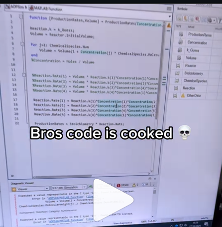
A coworker shared with me a hilarious Instagram post today. A brave bro posted a short video showing his MATLAB code… casually throwing 49,000 errors!
Surprisingly, the video went virial and recieved 250,000+ likes and 800+ comments. You really never know what the Instagram algorithm is thinking, but apparently “my code is absolutely cooked” is a universal developer experience 😂
Last note: Can someone please help this Bro fix his code?
Is it possible to display a variable value within the ThingSpeak plot area?
I’m currently developing a multi-platform viewer using Flutter to eliminate the hassle of manual channel setup. Instead of adding IDs one by one, the app uses your User API Key to automatically discover and list all your ThingSpeak channels instantly.
Key Highlights (Work in Progress):
- Automatic Sync: All your channels appear in seconds.
- Multi-platform: Built for Web, Android, Windows, and Linux.
- Privacy-Focused: Secure local storage for your API keys.
I can't believe someone put time into this ;-)

Hi everyone
I've been using ThingSpeak for several years now without an issue until last Thursday.
I have four ThingSpeak channels which are used by three Arduino devices (in two locations/on two distinct networks) all running the same code.
All three devices stopped being able to write data to my ThingSpeak channels around 17:00 CET on 4 Dec and are still unable to.
Nothing changed on this side, let alone something that would explain the problem.
I would note that data can still be written to all the channels via a browser so there is no fundamental problem with the channels (such as being full).
Since the above date and time, any HTTP/1.1 'update' (write) requests via the REST API (using both simple one-write GET requests or bulk JSON POST requests) are timing out after 5 seconds and no data is being written. The 5 second timeout is my Arduino code's default, but even increasing it to 30 seconds makes no difference. Before all this, responses from ThingSpeak were sub-second.
I have recompiled the Arduino code using the latest libraries and that didn't help.
I have tested the same code again another random api (api.ipify.org) and that works just fine.
Curl works just fine too, also usng HTTP/1.1
So the issue appears to be something particular to the combination of my Arduino code *and* the ThingSpeak environment, where something changed on the ThingSpeak end at the above date and time.
If anyone in the community has any suggestions as to what might be going on, I would greatly appreciate the help.
Peter

The formula comes from @yuruyurau. (https://x.com/yuruyurau)
digital life 1

figure('Position',[300,50,900,900], 'Color','k');
axes(gcf, 'NextPlot','add', 'Position',[0,0,1,1], 'Color','k');
axis([0, 400, 0, 400])
SHdl = scatter([], [], 2, 'filled','o','w', 'MarkerEdgeColor','none', 'MarkerFaceAlpha',.4);
t = 0;
i = 0:2e4;
x = mod(i, 100);
y = floor(i./100);
k = x./4 - 12.5;
e = y./9 + 5;
o = vecnorm([k; e])./9;
while true
t = t + pi/90;
q = x + 99 + tan(1./k) + o.*k.*(cos(e.*9)./4 + cos(y./2)).*sin(o.*4 - t);
c = o.*e./30 - t./8;
SHdl.XData = (q.*0.7.*sin(c)) + 9.*cos(y./19 + t) + 200;
SHdl.YData = 200 + (q./2.*cos(c));
drawnow
end
digital life 2

figure('Position',[300,50,900,900], 'Color','k');
axes(gcf, 'NextPlot','add', 'Position',[0,0,1,1], 'Color','k');
axis([0, 400, 0, 400])
SHdl = scatter([], [], 2, 'filled','o','w', 'MarkerEdgeColor','none', 'MarkerFaceAlpha',.4);
t = 0;
i = 0:1e4;
x = i;
y = i./235;
e = y./8 - 13;
while true
t = t + pi/240;
k = (4 + sin(y.*2 - t).*3).*cos(x./29);
d = vecnorm([k; e]);
q = 3.*sin(k.*2) + 0.3./k + sin(y./25).*k.*(9 + 4.*sin(e.*9 - d.*3 + t.*2));
SHdl.XData = q + 30.*cos(d - t) + 200;
SHdl.YData = 620 - q.*sin(d - t) - d.*39;
drawnow
end
digital life 3

figure('Position',[300,50,900,900], 'Color','k');
axes(gcf, 'NextPlot','add', 'Position',[0,0,1,1], 'Color','k');
axis([0, 400, 0, 400])
SHdl = scatter([], [], 1, 'filled','o','w', 'MarkerEdgeColor','none', 'MarkerFaceAlpha',.4);
t = 0;
i = 0:1e4;
x = mod(i, 200);
y = i./43;
k = 5.*cos(x./14).*cos(y./30);
e = y./8 - 13;
d = (k.^2 + e.^2)./59 + 4;
a = atan2(k, e);
while true
t = t + pi/20;
q = 60 - 3.*sin(a.*e) + k.*(3 + 4./d.*sin(d.^2 - t.*2));
c = d./2 + e./99 - t./18;
SHdl.XData = q.*sin(c) + 200;
SHdl.YData = (q + d.*9).*cos(c) + 200;
drawnow; pause(1e-2)
end
digital life 4

figure('Position',[300,50,900,900], 'Color','k');
axes(gcf, 'NextPlot','add', 'Position',[0,0,1,1], 'Color','k');
axis([0, 400, 0, 400])
SHdl = scatter([], [], 1, 'filled','o','w', 'MarkerEdgeColor','none', 'MarkerFaceAlpha',.4);
t = 0;
i = 0:4e4;
x = mod(i, 200);
y = i./200;
k = x./8 - 12.5;
e = y./8 - 12.5;
o = (k.^2 + e.^2)./169;
d = .5 + 5.*cos(o);
while true
t = t + pi/120;
SHdl.XData = x + d.*k.*sin(d.*2 + o + t) + e.*cos(e + t) + 100;
SHdl.YData = y./4 - o.*135 + d.*6.*cos(d.*3 + o.*9 + t) + 275;
SHdl.CData = ((d.*sin(k).*sin(t.*4 + e)).^2).'.*[1,1,1];
drawnow;
end
digital life 5

figure('Position',[300,50,900,900], 'Color','k');
axes(gcf, 'NextPlot','add', 'Position',[0,0,1,1], 'Color','k');
axis([0, 400, 0, 400])
SHdl = scatter([], [], 1, 'filled','o','w',...
'MarkerEdgeColor','none', 'MarkerFaceAlpha',.4);
t = 0;
i = 0:1e4;
x = mod(i, 200);
y = i./55;
k = 9.*cos(x./8);
e = y./8 - 12.5;
while true
t = t + pi/120;
d = (k.^2 + e.^2)./99 + sin(t)./6 + .5;
q = 99 - e.*sin(atan2(k, e).*7)./d + k.*(3 + cos(d.^2 - t).*2);
c = d./2 + e./69 - t./16;
SHdl.XData = q.*sin(c) + 200;
SHdl.YData = (q + 19.*d).*cos(c) + 200;
drawnow;
end
digital life 6

clc; clear
figure('Position',[300,50,900,900], 'Color','k');
axes(gcf, 'NextPlot','add', 'Position',[0,0,1,1], 'Color','k');
axis([0, 400, 0, 400])
SHdl = scatter([], [], 2, 'filled','o','w', 'MarkerEdgeColor','none', 'MarkerFaceAlpha',.4);
t = 0;
i = 1:1e4;
y = i./790;
k = y; idx = y < 5;
k(idx) = 6 + sin(bitxor(floor(y(idx)), 1)).*6;
k(~idx) = 4 + cos(y(~idx));
while true
t = t + pi/90;
d = sqrt((k.*cos(i + t./4)).^2 + (y/3-13).^2);
q = y.*k.*cos(i + t./4)./5.*(2 + sin(d.*2 + y - t.*4));
c = d./3 - t./2 + mod(i, 2);
SHdl.XData = q + 90.*cos(c) + 200;
SHdl.YData = 400 - (q.*sin(c) + d.*29 - 170);
drawnow; pause(1e-2)
end
digital life 7

clc; clear
figure('Position',[300,50,900,900], 'Color','k');
axes(gcf, 'NextPlot','add', 'Position',[0,0,1,1], 'Color','k');
axis([0, 400, 0, 400])
SHdl = scatter([], [], 2, 'filled','o','w', 'MarkerEdgeColor','none', 'MarkerFaceAlpha',.4);
t = 0;
i = 1:1e4;
y = i./345;
x = y; idx = y < 11;
x(idx) = 6 + sin(bitxor(floor(x(idx)), 8))*6;
x(~idx) = x(~idx)./5 + cos(x(~idx)./2);
e = y./7 - 13;
while true
t = t + pi/120;
k = x.*cos(i - t./4);
d = sqrt(k.^2 + e.^2) + sin(e./4 + t)./2;
q = y.*k./d.*(3 + sin(d.*2 + y./2 - t.*4));
c = d./2 + 1 - t./2;
SHdl.XData = q + 60.*cos(c) + 200;
SHdl.YData = 400 - (q.*sin(c) + d.*29 - 170);
drawnow; pause(5e-3)
end
digital life 8

clc; clear
figure('Position',[300,50,900,900], 'Color','k');
axes(gcf, 'NextPlot','add', 'Position',[0,0,1,1], 'Color','k');
axis([0, 400, 0, 400])
SHdl{6} = [];
for j = 1:6
SHdl{j} = scatter([], [], 2, 'filled','o','w', 'MarkerEdgeColor','none', 'MarkerFaceAlpha',.3);
end
t = 0;
i = 1:2e4;
k = mod(i, 25) - 12;
e = i./800; m = 200;
theta = pi/3;
R = [cos(theta) -sin(theta); sin(theta) cos(theta)];
while true
t = t + pi/240;
d = 7.*cos(sqrt(k.^2 + e.^2)./3 + t./2);
XY = [k.*4 + d.*k.*sin(d + e./9 + t);
e.*2 - d.*9 - d.*9.*cos(d + t)];
for j = 1:6
XY = R*XY;
SHdl{j}.XData = XY(1,:) + m;
SHdl{j}.YData = XY(2,:) + m;
end
drawnow;
end
digital life 9

clc; clear
figure('Position',[300,50,900,900], 'Color','k');
axes(gcf, 'NextPlot','add', 'Position',[0,0,1,1], 'Color','k');
axis([0, 400, 0, 400])
SHdl{14} = [];
for j = 1:14
SHdl{j} = scatter([], [], 2, 'filled','o','w', 'MarkerEdgeColor','none', 'MarkerFaceAlpha',.1);
end
t = 0;
i = 1:2e4;
k = mod(i, 50) - 25;
e = i./1100; m = 200;
theta = pi/7;
R = [cos(theta) -sin(theta); sin(theta) cos(theta)];
while true
t = t + pi/240;
d = 5.*cos(sqrt(k.^2 + e.^2) - t + mod(i, 2));
XY = [k + k.*d./6.*sin(d + e./3 + t);
90 + e.*d - e./d.*2.*cos(d + t)];
for j = 1:14
XY = R*XY;
SHdl{j}.XData = XY(1,:) + m;
SHdl{j}.YData = XY(2,:) + m;
end
drawnow;
end
Hello,
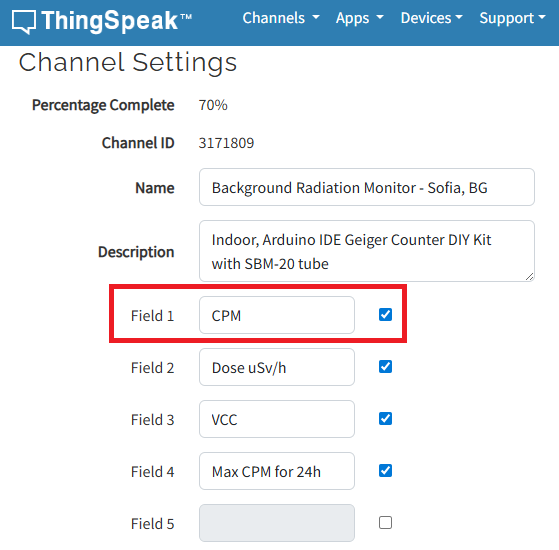
I have Arduino DIY Geiger Counter, that uploads data to my channel here in ThingSpeak (3171809), using ESP8266 WiFi board. It sends CPM values (counts per minute), Dose, VCC and Max CPM for 24h. They are assignet to Field from 1 to 4 respectively. How can I duplicate Field 1, so I could create different time chart for the same measured unit? Or should I duplicate Field 1 chart, and how? I tried to find the answer here in the blog, but I couldn't.
I have to say that I'm not an engineer or coder, just can simply load some Arduino sketches and few more things, so I'll be very thankfull if someone could explain like for non-IT users.
Regards,
Emo
Pure Matlab
82%
Simulink
18%
11 votes
Jorge Bernal-AlvizJorge Bernal-Alviz shared the following code that requires R2025a or later:
Test()

function Test()
duration = 10;
numFrames = 800;
frameInterval = duration / numFrames;
w = 400;
t = 0;
i_vals = 1:10000;
x_vals = i_vals;
y_vals = i_vals / 235;
r = linspace(0, 1, 300)';
g = linspace(0, 0.1, 300)';
b = linspace(1, 0, 300)';
r = r * 0.8 + 0.1;
g = g * 0.6 + 0.1;
b = b * 0.9 + 0.1;
customColormap = [r, g, b];
figure('Position', [100, 100, w, w], 'Color', [0, 0, 0]);
axis equal;
axis off;
xlim([0, w]);
ylim([0, w]);
hold on;
colormap default;
colormap(customColormap);
plothandle = scatter([], [], 1, 'filled', 'MarkerFaceAlpha', 0.12);
for i = 1:numFrames
t = t + pi/240;
k = (4 + 3 * sin(y_vals * 2 - t)) .* cos(x_vals / 29);
e = y_vals / 8 - 13;
d = sqrt(k.^2 + e.^2);
c = d - t;
q = 3 * sin(2 * k) + 0.3 ./ (k + 1e-10) + ...
sin(y_vals / 25) .* k .* (9 + 4 * sin(9 * e - 3 * d + 2 * t));
points_x = q + 30 * cos(c) + 200;
points_y = q .* sin(c) + 39 * d - 220;
points_y = w - points_y;
CData = (1 + sin(0.1 * (d - t))) / 3;
CData = max(0, min(1, CData));
set(plothandle, 'XData', points_x, 'YData', points_y, 'CData', CData);
brightness = 0.5 + 0.3 * sin(t * 0.2);
set(plothandle, 'MarkerFaceAlpha', brightness);
drawnow;
pause(frameInterval);
end
end
как я получил api Token
Hey everyone,
I’m currently working with MATLAB R2025b and using the MQTT blocks from the Industrial Communication Toolbox inside Simulink. I’ve run into an issue that’s driving me a bit crazy, and I’m not sure if it’s a bug or if I’m missing something obvious.
Here’s what’s happening:
- I open the MQTT Configure block.
- I fill out all the required fields — Broker address, Port, Client ID, Username, and Password.
- When I click Test Connection, it says “Connection established successfully.” So far so good.
- Then I click Apply, close the dialog, set the topic name, and try to run the simulation.
- At this point, I get the following error:Caused by: Invalid value for 'ClientID', 'Username' or 'Password'.
- When I reopen the MQTT config block, I notice that the Password field is empty again — even though I definitely entered it before and the connection test worked earlier.
It seems like Simulink is somehow not saving the password after hitting Apply, which leads to the authentication error during simulation.
Has anyone else faced this? Is this a bug in R2025b, or do I need to configure something differently to make the password persist?
Would really appreciate any insights, workarounds, or confirmations from anyone who has used MQTT in Simulink recently.
Thanks in advance!