Main Content

Results for

Hello,
I have Arduino DIY Geiger Counter, that uploads data to my channel here in ThingSpeak (3171809), using ESP8266 WiFi board. It sends CPM values (counts per minute), Dose, VCC and Max CPM for 24h. They are assignet to Field from 1 to 4 respectively. How can I duplicate Field 1, so I could create different time chart for the same measured unit? Or should I duplicate Field 1 chart, and how? I tried to find the answer here in the blog, but I couldn't.
I have to say that I'm not an engineer or coder, just can simply load some Arduino sketches and few more things, so I'll be very thankfull if someone could explain like for non-IT users.
Regards,
Emo
Matt Tearle
Matt Tearle
Last activity on 13 Dec 2025 at 11:50

Fittingly for a Creative Coder, @Vasilis Bellos clearly enjoyed the silliness I put into the problems. If you've solved the whole problem set, don't forget to help out your teammates with suggestions, tips, tricks, etc. But also, just for fun, I'm curious to see which of my many in-jokes and nerdy references you noticed. Many of the problems were inspired by things in the real world, then ported over into the chaotic fantasy world of Nedland.
I guess I'll start with the obvious real-world reference: @Ned Gulley (I make no comment about his role as insane despot in any universe, real or otherwise.)
Experimenting with Agentic AI
44%
I am an AI skeptic
0%
AI is banned at work
11%
I am happy with Conversational AI
44%
9 votes
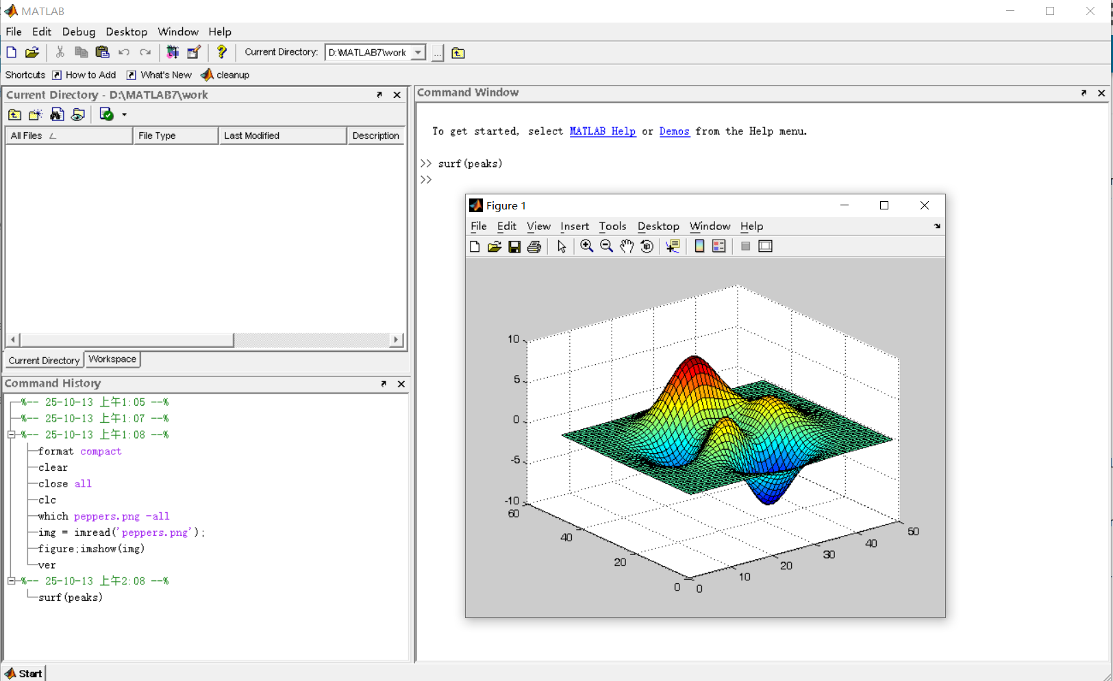
The Cody Contest 2025 is underway, and it includes a super creative problem group which many of us have found fascinating. The central theme of the problems, expertly curated by @Matt Tearle, humorously revolves around the whims of the capricious dictator Lord Ned, as he goes out of his way to complicate the lives of his subjects and visitors alike. We cannot judge whether or not there's any truth to the rumors behind all the inside jokes, but it's obvious that the team had a lot of fun creating these; and we had even more fun solving them.
Today I want to showcase a way of graphically solving and visualizing one of those problems which I found very elegant, The Bridges of Nedsburg.
To briefly reiterate the problem, the number of islands and the arrangement of bridges of the city of Nedsburg are constantly changing. Lord Ned has decided to take advantage of this by charging visitors with an increasingly expensive n-bridge pass which allows them to cross up to n bridges in one journey. Given the Connectivity Matrix C, we are tasked with calculating the minimum n needed so that there is a path from every island to every other island in n steps or fewer.
Matt kindly provided us with some useful bit of math in the description detailing how to calculate the way to get from one island to another in an number of m steps. However, he has also hidden an alternative path to the solution in plain sight, in one of the graphs he provided. This involves the extremely useful and versatile class digraph, representing directed graphs, which have directional edges connecting the nodes. Here's some further great documentation and other cool resources on the topic for those who are interested in learning more about it:
Let's start using this class to explore a graphical solution to Lord Ned's conundrum. We will use the unit tests included in the problem to visualize the solution. We can retrieve the connectivity matrix for each case using the following function:
function C = getConnectivityMatrix(unit_test)
% Number of islands and bridge arrangement
switch unit_test
case 1
m = 3; idx = [3;4;8];
case 2
m = 3; idx = [3;4;7;8];
case 3
m = 4; idx = [2;7;8;10;13];
case 4
m = 4; idx = [4;5;7;8;9;14];
case 5
m = 5; idx = [5;8;11;12;14;18;22;23];
case 6
m = 5; idx = [2;5;8;14;20;21;24];
case 7
m = 6; idx = [3;4;7;11;18;23;24;26;30;32];
case 8
m = 6; idx = [3;11;12;13;18;19;28;32];
case 9
m = 7; idx = [3;4;6;8;13;14;20;21;23;31;36;47];
case 10
m = 7; idx = [4;11;13;14;19;22;23;26;28;30;34;35;37;38;45];
case 11
m = 8; idx = [2;4;5;6;8;12;13;17;27;39;44;48;54;58;60;62];
case 12
m = 8; idx = [3;9;12;20;24;29;30;31;33;44;48;50;53;54;58];
case 13
m = 9; idx = [8;9;10;14;15;22;25;26;29;33;36;42;44;47;48;50;53;54;55;67;80];
case 14
m = 9; idx = [8;10;22;32;37;40;43;45;47;53;56;57;62;64;69;70;73;77;79];
case 15
m = 10; idx = [2;5;8;13;16;20;24;27;28;36;43;49;53;62;71;75;77;83;86;87;95];
case 16
m = 10; idx = [4;9;14;21;22;35;37;38;44;47;50;51;53;55;59;61;63;66;69;76;77;84;85;86;90;97];
end
C = zeros(m);
C(idx) = 1;
end
The case in the example refers to unit test case 2.
unit_test = 2;
C = getConnectivityMatrix(unit_test);
disp(C)
0 1 1 0 0 1 1 0 0
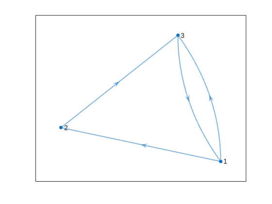
We can now create a digraph object D, and visualize it using its corresponding plot method:
D = digraph(C);
figure
p = plot(D,'LineWidth',1.5,'ArrowSize',10);
This is the same as the graph provided in the example. Another very useful method of digraph is shortestpath. This allows us to calculate the path and distance from one single node to another. For example:
% Path and distance from node 1 to node 2
[path12,dist12] = shortestpath(D,1,2);
fprintf('The shortest path from island %d to island %d is: %s. The minimum number of steps is: n = %d\n', 1, 2, join(string(path12), ' -> '),dist12)
The shortest path from island 1 to island 2 is: 1 -> 2. The minimum number of steps is: n = 1
% Path and distance from node 2 to node 1
[path21,dist21] = shortestpath(D,2,1);
fprintf('The shortest path from island %d to island %d is: %s. The minimum number of steps is: n = %d\n', 2, 1, join(string(path21), ' -> '),dist21)
The shortest path from island 2 to island 1 is: 2 -> 3 -> 1. The minimum number of steps is: n = 2
We can visualize these using the highlight method of the graph plot:
figure
p = plot(D,'LineWidth',1.5,'ArrowSize',10);
highlight(p,path12,'EdgeColor','r','NodeColor','r','LineWidth',2)
highlight(p,path21,'EdgeColor',[0 0.8 0],'LineWidth',2)
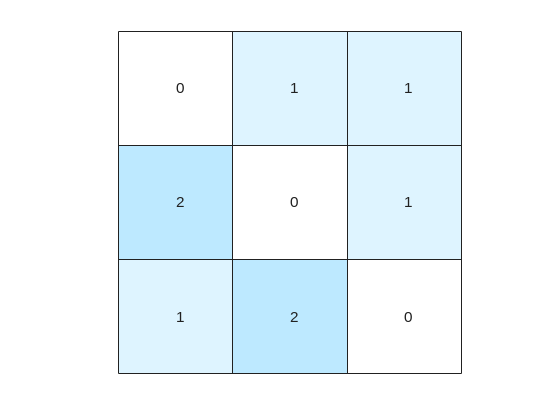
But that's not all! digraph can also provide us with a matrix of the distances d, i.e. the steps needed to travel from island i to island j, where i and j are the rows and columns of d respectively. This is accomplished by using its distances method. The distance matrix can be visualized as:
d = distances(D);
figure
% Using pcolor w/ appending matrix workaround for convenience
pcolor([d,d(:,end);d(end,:),d(end,end)])
% Alternatively you can use imagesc(d), but you'll have to recreate the grid manually
axis square
set(gca,'YDir','reverse','XTick',[],'YTick',[])
[X,Y] = meshgrid(1:height(d));
text(X(:)+0.5,Y(:)+0.5,string(d(:)),'FontSize',11)
colormap(interp1(linspace(0,1,4), [1 1 1; 0.7 0.9 1; 0.6 0.7 1; 1 0.3 0.3], linspace(0,1,8)))
clim([-0.5 7+0.5])
This confirms what we saw before, i.e. you need 1 step to go from island 1 to island 2, but 2 steps for vice versa. It also confirms that the minimum number of steps n that you need to buy the pass for is 2 (which also occurs for traveling from island 3 to island 2). As it's not the point of the post to give the full solution to the problem but rather present the graphical way of visualizing it I will not include the code of how to calculate this, but I'm sure that by now it's reduced to a trivial problem which you have already figured out how to solve.
That being said, now that we have the distance matrix, let's continue with the visualizations. First, let's plot the corresponding paths for each of these combinations:
figure
tiledlayout(size(C,1),size(C,2),'TileSpacing','tight','Padding','tight');
for i = 1:size(C,1)
for j = 1:size(C,2)
nexttile
p = plot(D,'ArrowSize',10);
highlight(p,shortestpath(D,i,j),'EdgeColor','r','NodeColor','r','LineWidth',2)
lims = axis;
text(lims(1)+diff(lims(1:2))*0.05,lims(3)+diff(lims(3:4))*0.9,sprintf('n = %d',d(i,j)))
end
end
This allows us to go from the distance matrix to visualizing the paths and number of steps for each corresponding case. Things are rather simple for this 3-island example case, but evil Lord Ned is just getting started. Let's now try to solve the problem for all provided unit test cases:
% Cell array of connectivity matrices
C = arrayfun(@getConnectivityMatrix,1:16,'UniformOutput',false);
% Cell array of corresponding digraph objects
D = cellfun(@digraph,C,'UniformOutput',false);
% Cell array of corresponding distance matrices
d = cellfun(@distances,D,'UniformOutput',false);
% id of solutions: Provided as is to avoid handing out the code to the full solution
id = [2, 2, 9, 3, 4, 6, 16, 4, 44, 43, 33, 34, 7, 18, 39, 2];
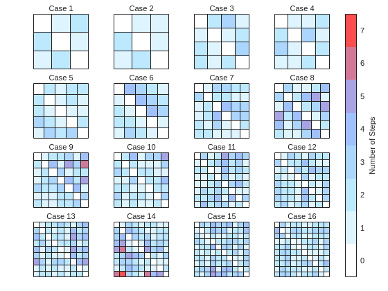
First, let's plot the distance matrix for each case:
figure
tiledlayout('flow','TileSpacing','compact','Padding','compact');
% Vary this to plot different combinations of cases
plot_cases = 1:numel(C);
for i = plot_cases
nexttile
pcolor([d{i},d{i}(:,end);d{i}(end,:),d{i}(end,end)])
axis square
set(gca,'YDir','reverse','XTick',[],'YTick',[])
title(sprintf('Case %d',i),'FontWeight','normal','FontSize',8)
end
c = colorbar('Ticks',0:7,'TickLength',0,'Limits',[-0.5 7+0.5],'FontSize',8);
c.Layout.Tile = 'East';
c.Label.String = 'Number of Steps';
c.Label.FontSize = 8;
colormap(interp1(linspace(0,1,4), [1 1 1; 0.7 0.9 1; 0.6 0.7 1; 1 0.3 0.3], linspace(0,1,8)))
clim(findobj(gcf,'type','axes'),[-0.5 7+0.5])
We immediately notice some inconsistencies, perhaps to be expected of the eccentric and cunning dictator. Things are pretty simple for the configurations with a small number of islands, but the minimum number of steps n can increase sharply and disproportionally to the additional number of islands. Cases 8 and 9 specifically have a particularly large n (relative to their grid dimensions), and case 14 has the largest n, almost double that of case 16 despite the fact that the latter has one extra island.
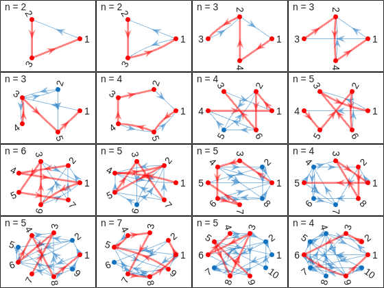
To visualize how this is possible, let's plot the path corresponding to the largest n for each case (though note that there might be multiple possible paths for each case):
figure
tiledlayout('flow','TileSpacing','tight','Padding','tight');
for i = plot_cases
nexttile
% Changing the layout to circular so we can better visualize the paths
p = plot(D{i},'ArrowSize',10,'Layout','Circle');
% Alternatively we could use the XData and YData properties if the positions of the islands were provided
axis([-1.5 1.5 -1.5 1.75])
[row,col] = ind2sub(size(d{i}),id(i));
highlight(p,shortestpath(D{i},row,col),'EdgeColor','r','NodeColor','r','LineWidth',2)
lims = axis;
text(lims(1)+diff(lims(1:2))*0.05,lims(3)+diff(lims(3:4))*0.9,sprintf('n = %d',d{i}(row,col)))
end
And busted! Unraveled! Exposed! Lord Ned has clearly been taking advantages of the tectonic forces by instructing his corrupt civil engineer lackeys to design the bridges to purposely force the visitors to go around in circles in order to drain them of their precious savings. In particular, for cases 8 and 9, he would have them go through every single island just to get from one island to another, whereas for case 14 they would have to visit 8 of the 9 islands just to get to their destination. If that's not diabolical then I don't know what is!
Ned jokes aside, I hope you enjoyed this contest just as much as I did, and that you found this article useful. I look forward to seeing more creative problems and solutions in the future.
It’s exciting to dive into a new dataset full of unfamiliar variables but it can also be overwhelming if you’re not sure where to start. Recently, I discovered some new interactive features in MATLAB live scripts that make it much easier to get an overview of your data. With just a few clicks, you can display sparklines and summary statistics using table variables, sort and filter variables, and even have MATLAB generate the corresponding code for reproducibility.
The Graphics and App Building blog published an article that walks through these features showing how to explore, clean, and analyze data—all without writing any code.
If you’re interested in streamlining your exploratory data analysis or want to see what’s new in live scripts, you might find it helpful:
If you’ve tried these features or have your own tips for quick data exploration in MATLAB, I’d love to hear your thoughts!
Ludvig Nordin
Ludvig Nordin
Last activity on 13 Nov 2025

Pure Matlab
82%
Simulink
18%
11 votes
Jorge Bernal-AlvizJorge Bernal-Alviz shared the following code that requires R2025a or later:
Test()
Warning: Hardware-accelerated graphics is unavailable. Displaying fewer markers to preserve interactivity.
function Test()
duration = 10;
numFrames = 800;
frameInterval = duration / numFrames;
w = 400;
t = 0;
i_vals = 1:10000;
x_vals = i_vals;
y_vals = i_vals / 235;
r = linspace(0, 1, 300)';
g = linspace(0, 0.1, 300)';
b = linspace(1, 0, 300)';
r = r * 0.8 + 0.1;
g = g * 0.6 + 0.1;
b = b * 0.9 + 0.1;
customColormap = [r, g, b];
figure('Position', [100, 100, w, w], 'Color', [0, 0, 0]);
axis equal;
axis off;
xlim([0, w]);
ylim([0, w]);
hold on;
colormap default;
colormap(customColormap);
plothandle = scatter([], [], 1, 'filled', 'MarkerFaceAlpha', 0.12);
for i = 1:numFrames
t = t + pi/240;
k = (4 + 3 * sin(y_vals * 2 - t)) .* cos(x_vals / 29);
e = y_vals / 8 - 13;
d = sqrt(k.^2 + e.^2);
c = d - t;
q = 3 * sin(2 * k) + 0.3 ./ (k + 1e-10) + ...
sin(y_vals / 25) .* k .* (9 + 4 * sin(9 * e - 3 * d + 2 * t));
points_x = q + 30 * cos(c) + 200;
points_y = q .* sin(c) + 39 * d - 220;
points_y = w - points_y;
CData = (1 + sin(0.1 * (d - t))) / 3;
CData = max(0, min(1, CData));
set(plothandle, 'XData', points_x, 'YData', points_y, 'CData', CData);
brightness = 0.5 + 0.3 * sin(t * 0.2);
set(plothandle, 'MarkerFaceAlpha', brightness);
drawnow;
pause(frameInterval);
end
end
From my experience, MATLAB's Deep Learning Toolbox is quite user-friendly, but it still falls short of libraries like PyTorch in many respects. Most users tend to choose PyTorch because of its flexibility, efficiency, and rich support for many mathematical operators. In recent years, the number of dlarray-compatible mathematical functions added to the toolbox has been very limited, which makes it difficult to experiment with many custom networks. For example, svd is currently not supported for dlarray inputs.
This link (List of Functions with dlarray Support - MATLAB & Simulink) lists all functions that support dlarray as of R2026a — only around 200 functions (including toolbox-specific ones). I would like to see support for many more fundamental mathematical functions so that users have greater freedom when building and researching custom models. For context, the core MATLAB mathematics module contains roughly 600 functions, and many application domains build on that foundation.
I hope MathWorks will prioritize and accelerate expanding dlarray support for basic math functions. Doing so would significantly increase the Deep Learning Toolbox's utility and appeal for researchers and practitioners.
Thank you.
Run MATLAB using AI applications by leveraging MCP. This MCP server for MATLAB supports a wide range of coding agents like Claude Code and Visual Studio Code.
Check it out and share your experiences below. Have fun!
Hey Creative Coders! 😎
Let’s get to know each other. Drop a quick intro below and meet your teammates! This is your chance to meet teammates, find coding buddies, and build connections that make the contest more fun and rewarding!
You can share:
  • Your name or nickname
  • Where you’re from
  • Your favorite coding topic or language
  • What you’re most excited about in the contest
Let’s make Team Creative Coders an awesome community—jump in and say hi! 🚀
Welcome to the Cody Contest 2025 and the Creative Coders team channel! 🎉
You think outside the box. Where others see limitations, you see opportunities for innovation. This is your space to connect with like-minded coders, share insights, and help your team win. To make sure everyone has a great experience, please keep these tips in mind:
  1. Follow the Community Guidelines: Take a moment to review our community standards. Posts that don’t follow these guidelines may be flagged by moderators or community members.
  2. Ask Questions About Cody Problems: When asking for help, show your work! Include your code, error messages, and any details needed to reproduce your results. This helps others provide useful, targeted answers.
  3. Share Tips & Tricks: Knowledge sharing is key to success. When posting tips or solutions, explain how and why your approach works so others can learn your problem-solving methods.
  4. Provide Feedback: We value your feedback! Use this channel to report issues or share creative ideas to make the contest even better.
Have fun and enjoy the challenge! We hope you’ll learn new MATLAB skills, make great connections, and win amazing prizes! 🚀
как я получил api Token
David
David
Last activity on 8 Dec 2025 at 15:44

I just learned you can access MATLAB Online from the following shortcut in your web browser: https://matlab.new
Hey everyone,
I’m currently working with MATLAB R2025b and using the MQTT blocks from the Industrial Communication Toolbox inside Simulink. I’ve run into an issue that’s driving me a bit crazy, and I’m not sure if it’s a bug or if I’m missing something obvious.
Here’s what’s happening:
  • I open the MQTT Configure block.
  • I fill out all the required fields — Broker address, Port, Client ID, Username, and Password.
  • When I click Test Connection, it says “Connection established successfully.” So far so good.
  • Then I click Apply, close the dialog, set the topic name, and try to run the simulation.
  • At this point, I get the following error:Caused by: Invalid value for 'ClientID', 'Username' or 'Password'.
  • When I reopen the MQTT config block, I notice that the Password field is empty again — even though I definitely entered it before and the connection test worked earlier.
It seems like Simulink is somehow not saving the password after hitting Apply, which leads to the authentication error during simulation.
Has anyone else faced this? Is this a bug in R2025b, or do I need to configure something differently to make the password persist?
Would really appreciate any insights, workarounds, or confirmations from anyone who has used MQTT in Simulink recently.
Thanks in advance!
I'm working on training neural networks without backpropagation / automatic differentiation, using locally derived analytic forms of update rules. Given that this allows a direct formula to be derived for the update rule, it removes alot of the overhead that is otherwise required from automatic differentiation.
However, matlab's functionalities for neural networks are currently solely based around backpropagation and automatic differentiation, such as the dlgradient function and requiring everything to be dlarrays during training.
I have two main requests, specifically for functions that perform a single operation within a single layer of a neural network, such as "dlconv", "fullyconnect", "maxpool", "avgpool", "relu", etc:
  • these functions should also allow normal gpuArray data instead of requiring everything to be dlarrays.
  • these functions are currently designed to only perform the forward pass. I request that these also be designed to perform the backward pass if user requests. There can be another input user flag that can be "forward" (default) or "backward", and then the function should have all the necessary inputs to perform that operation (e.g. for "avgpool" forward pass it only needs the avgpool input data and the avgpool parameters, but for the "avgpool" backward pass it needs the deriviative w.r.t. the avgpool output data, the avgpool parameters, and the original data dimensions). I know that there is a maxunpool function that achieves this for maxpool, but it has significant issues when trying to use it this way instead of by backpropagation in a dlgradient type layer, see (https://www.mathworks.com/matlabcentral/answers/2179587-making-a-custom-way-to-train-cnns-and-i-am-noticing-that-avgpool-is-significantly-faster-than-maxpo?s_tid=srchtitle).
I don't know how many people would benefit from this feature, and someone could always spend their time creating these functionalities themselves by matlab scripts, cuDNN mex, etc., but regardless it would be nice for matlab to have this allowable for more customizable neural net training.
Inspired by @xingxingcui's post about old MATLAB versions and @유장's post about an old Easter egg, I thought it might be fun to share some MATLAB-Old-Timer Stories™.
Back in the early 90s, MATLAB had been ported to MacOS, but there were some interesting wrinkles. One that kept me earning my money as a computer lab tutor was that MATLAB required file names to follow Windows standards - no spaces or other special characters. But on a Mac, nothing stopped you from naming your script "hello world - 123.m". The problem came when you tried to run it. MATLAB was essentially doing an eval on the script name, assuming the file name would follow Windows (and MATLAB) naming rules.
So now imagine a lab full of students taking a university course. As is common in many universities, the course was given a numeric code. For whatever historical reason, my school at that time was also using numeric codes for the departments. Despite being told the rules for naming scripts, many students would default to something like "26.165 - 1.1" for problem one on HW1 for the intro applied math course 26.165.
No matter what they did in their script, when they ran it, MATLAB would just say "ans = 25.0650".
Nothing brings you more MATLAB-god credibility as a student tutor than walking over to someone's computer, taking one look at their output, saying "rename your file", and walking away like a boss.
It was 2010 when I was a sophomore in university. I chose to learn MATLAB because of a mathematical modeling competition, and the university provided MATLAB 7.0, a very classic release. To get started, I borrowed many MATLAB books from the library and began by learning simple numerical calculations, plotting, and solving equations. Gradually I was drawn in by MATLAB’s powerful capabilities and became interested; I often used it as a big calculator for fun. That version didn’t have MATLAB Live Script; instead it used MATLAB Notebook (M-Book), which allowed MATLAB functions to be used directly within Microsoft Word, and it also had the Symbolic Math Toolbox’s MuPAD interactive environment. These were later gradually replaced by Live Scripts introduced in R2016a. There are many similar examples...
Out of curiosity, I still have screenshots on my computer showing MATLAB 7.0 running compatibly. I’d love to hear your thoughts?
Edit 15 Oct 2025: Removed incorrect code. Replaced symmatrix2sym and symfunmatrix2symfun with sym and symfun respectively (latter supported as of 2024b).
The Symbolic Math Toolbox does not have its own dot and and cross functions. That's o.k. (maybe) for garden variety vectors of sym objects where those operations get shipped off to the base Matlab functions
x = sym('x',[3,1]); y = sym('y',[3,1]);
which dot(x,y)
/MATLAB/toolbox/matlab/specfun/dot.m
dot(x,y)
ans = 
which cross(x,y)
/MATLAB/toolbox/matlab/specfun/cross.m
cross(x,y)
ans = 
But now we have symmatrix et. al., and things don't work as nicely
clearvars
x = symmatrix('x',[3,1]); y = symmatrix('y',[3,1]);
z = symmatrix('z',[1,1]);
sympref('AbbreviateOutput',false);
dot() expands the result, which isn't really desirable for exposition.
eqn = z == dot(x,y)
eqn = 
Also, dot() returns the the result in terms of the conjugate of x, which can't be simplifed away at the symmatrix level
assumeAlso(sym(x),'real')
class(eqn)
ans = 'symmatrix'
try
eqn = z == simplify(dot(x,y))
catch ME
ME.message
end
ans = 'Undefined function 'simplify' for input arguments of type 'symmatrix'.'
To get rid of the conjugate, we have to resort to sym
eqn = simplify(sym(eqn))
eqn = 
but again we are in expanded form, which defeats the purpose of symmatrix (et. al.)
But at least we can do this to get a nice equation
eqn = z == x.'*y
eqn = 
dot errors with symfunmatrix inputs
clearvars
syms t real
x = symfunmatrix('x(t)',t,[3,1]); y = symfunmatrix('y(t)',t,[3,1]);
try
dot(x,y)
catch ME
ME.message
end
ans = 'Invalid argument at position 2. Symbolic function is evaluated at the input arguments and does not accept colon indexing. Instead, use FORMULA on the function and perform colon indexing on the returned output.'
Cross works (accidentally IMO) with symmatrix, but expands the result, which isn't really desirable for exposition
clearvars
x = symmatrix('x',[3,1]); y = symmatrix('y',[3,1]);
z = symmatrix('z',[3,1]);
eqn = z == cross(x,y)
eqn = 
And it doesn't work at all if an input is a symfunmatrix
syms t
w = symfunmatrix('w(t)',t,[3,1]);
try
eqn = z == cross(x,w);
catch ME
ME.message
end
ans = 'A and B must be of length 3 in the dimension in which the cross product is taken.'
In the latter case we can expand with
eqn = z == cross(sym(x),symfun(w)) % x has to be converted
eqn(t) = 
But we can't do the same with dot (as shown above, dot doesn't like symfun inputs)
try
eqn = z == dot(sym(x),symfun(w))
catch ME
ME.message
end
ans = 'Invalid argument at position 2. Symbolic function is evaluated at the input arguments and does not accept colon indexing. Instead, use FORMULA on the function and perform colon indexing on the returned output.'
Looks like the only choice for dot with symfunmatrix is to write it by hand at the matrix level
x.'*w
ans(t) = 
or at the sym/symfun level
sym(x).'*symfun(w) % assuming x is real
ans(t) = 
Ideally, I'd like to see dot and cross implemented for symmatrix and symfunmatrix types where neither function would evaluate, i.e., expand, until both arguments are subs-ed with sym or symfun objects of appropriate dimension.
Also, it would be nice if symmatrix could be assumed to be real. Is there a reason why being able to do so wouldn't make sense?
try
assume(x,'real')
catch ME
ME.message
end
ans = 'Undefined function 'assume' for input arguments of type 'symmatrix'.'