Results for

The formula comes from @yuruyurau. (https://x.com/yuruyurau)
digital life 1

figure('Position',[300,50,900,900], 'Color','k');
axes(gcf, 'NextPlot','add', 'Position',[0,0,1,1], 'Color','k');
axis([0, 400, 0, 400])
SHdl = scatter([], [], 2, 'filled','o','w', 'MarkerEdgeColor','none', 'MarkerFaceAlpha',.4);
t = 0;
i = 0:2e4;
x = mod(i, 100);
y = floor(i./100);
k = x./4 - 12.5;
e = y./9 + 5;
o = vecnorm([k; e])./9;
while true
t = t + pi/90;
q = x + 99 + tan(1./k) + o.*k.*(cos(e.*9)./4 + cos(y./2)).*sin(o.*4 - t);
c = o.*e./30 - t./8;
SHdl.XData = (q.*0.7.*sin(c)) + 9.*cos(y./19 + t) + 200;
SHdl.YData = 200 + (q./2.*cos(c));
drawnow
end
digital life 2

figure('Position',[300,50,900,900], 'Color','k');
axes(gcf, 'NextPlot','add', 'Position',[0,0,1,1], 'Color','k');
axis([0, 400, 0, 400])
SHdl = scatter([], [], 2, 'filled','o','w', 'MarkerEdgeColor','none', 'MarkerFaceAlpha',.4);
t = 0;
i = 0:1e4;
x = i;
y = i./235;
e = y./8 - 13;
while true
t = t + pi/240;
k = (4 + sin(y.*2 - t).*3).*cos(x./29);
d = vecnorm([k; e]);
q = 3.*sin(k.*2) + 0.3./k + sin(y./25).*k.*(9 + 4.*sin(e.*9 - d.*3 + t.*2));
SHdl.XData = q + 30.*cos(d - t) + 200;
SHdl.YData = 620 - q.*sin(d - t) - d.*39;
drawnow
end
digital life 3

figure('Position',[300,50,900,900], 'Color','k');
axes(gcf, 'NextPlot','add', 'Position',[0,0,1,1], 'Color','k');
axis([0, 400, 0, 400])
SHdl = scatter([], [], 1, 'filled','o','w', 'MarkerEdgeColor','none', 'MarkerFaceAlpha',.4);
t = 0;
i = 0:1e4;
x = mod(i, 200);
y = i./43;
k = 5.*cos(x./14).*cos(y./30);
e = y./8 - 13;
d = (k.^2 + e.^2)./59 + 4;
a = atan2(k, e);
while true
t = t + pi/20;
q = 60 - 3.*sin(a.*e) + k.*(3 + 4./d.*sin(d.^2 - t.*2));
c = d./2 + e./99 - t./18;
SHdl.XData = q.*sin(c) + 200;
SHdl.YData = (q + d.*9).*cos(c) + 200;
drawnow; pause(1e-2)
end
digital life 4

figure('Position',[300,50,900,900], 'Color','k');
axes(gcf, 'NextPlot','add', 'Position',[0,0,1,1], 'Color','k');
axis([0, 400, 0, 400])
SHdl = scatter([], [], 1, 'filled','o','w', 'MarkerEdgeColor','none', 'MarkerFaceAlpha',.4);
t = 0;
i = 0:4e4;
x = mod(i, 200);
y = i./200;
k = x./8 - 12.5;
e = y./8 - 12.5;
o = (k.^2 + e.^2)./169;
d = .5 + 5.*cos(o);
while true
t = t + pi/120;
SHdl.XData = x + d.*k.*sin(d.*2 + o + t) + e.*cos(e + t) + 100;
SHdl.YData = y./4 - o.*135 + d.*6.*cos(d.*3 + o.*9 + t) + 275;
SHdl.CData = ((d.*sin(k).*sin(t.*4 + e)).^2).'.*[1,1,1];
drawnow;
end
digital life 5

figure('Position',[300,50,900,900], 'Color','k');
axes(gcf, 'NextPlot','add', 'Position',[0,0,1,1], 'Color','k');
axis([0, 400, 0, 400])
SHdl = scatter([], [], 1, 'filled','o','w',...
'MarkerEdgeColor','none', 'MarkerFaceAlpha',.4);
t = 0;
i = 0:1e4;
x = mod(i, 200);
y = i./55;
k = 9.*cos(x./8);
e = y./8 - 12.5;
while true
t = t + pi/120;
d = (k.^2 + e.^2)./99 + sin(t)./6 + .5;
q = 99 - e.*sin(atan2(k, e).*7)./d + k.*(3 + cos(d.^2 - t).*2);
c = d./2 + e./69 - t./16;
SHdl.XData = q.*sin(c) + 200;
SHdl.YData = (q + 19.*d).*cos(c) + 200;
drawnow;
end
digital life 6

clc; clear
figure('Position',[300,50,900,900], 'Color','k');
axes(gcf, 'NextPlot','add', 'Position',[0,0,1,1], 'Color','k');
axis([0, 400, 0, 400])
SHdl = scatter([], [], 2, 'filled','o','w', 'MarkerEdgeColor','none', 'MarkerFaceAlpha',.4);
t = 0;
i = 1:1e4;
y = i./790;
k = y; idx = y < 5;
k(idx) = 6 + sin(bitxor(floor(y(idx)), 1)).*6;
k(~idx) = 4 + cos(y(~idx));
while true
t = t + pi/90;
d = sqrt((k.*cos(i + t./4)).^2 + (y/3-13).^2);
q = y.*k.*cos(i + t./4)./5.*(2 + sin(d.*2 + y - t.*4));
c = d./3 - t./2 + mod(i, 2);
SHdl.XData = q + 90.*cos(c) + 200;
SHdl.YData = 400 - (q.*sin(c) + d.*29 - 170);
drawnow; pause(1e-2)
end
digital life 7

clc; clear
figure('Position',[300,50,900,900], 'Color','k');
axes(gcf, 'NextPlot','add', 'Position',[0,0,1,1], 'Color','k');
axis([0, 400, 0, 400])
SHdl = scatter([], [], 2, 'filled','o','w', 'MarkerEdgeColor','none', 'MarkerFaceAlpha',.4);
t = 0;
i = 1:1e4;
y = i./345;
x = y; idx = y < 11;
x(idx) = 6 + sin(bitxor(floor(x(idx)), 8))*6;
x(~idx) = x(~idx)./5 + cos(x(~idx)./2);
e = y./7 - 13;
while true
t = t + pi/120;
k = x.*cos(i - t./4);
d = sqrt(k.^2 + e.^2) + sin(e./4 + t)./2;
q = y.*k./d.*(3 + sin(d.*2 + y./2 - t.*4));
c = d./2 + 1 - t./2;
SHdl.XData = q + 60.*cos(c) + 200;
SHdl.YData = 400 - (q.*sin(c) + d.*29 - 170);
drawnow; pause(5e-3)
end
digital life 8

clc; clear
figure('Position',[300,50,900,900], 'Color','k');
axes(gcf, 'NextPlot','add', 'Position',[0,0,1,1], 'Color','k');
axis([0, 400, 0, 400])
SHdl{6} = [];
for j = 1:6
SHdl{j} = scatter([], [], 2, 'filled','o','w', 'MarkerEdgeColor','none', 'MarkerFaceAlpha',.3);
end
t = 0;
i = 1:2e4;
k = mod(i, 25) - 12;
e = i./800; m = 200;
theta = pi/3;
R = [cos(theta) -sin(theta); sin(theta) cos(theta)];
while true
t = t + pi/240;
d = 7.*cos(sqrt(k.^2 + e.^2)./3 + t./2);
XY = [k.*4 + d.*k.*sin(d + e./9 + t);
e.*2 - d.*9 - d.*9.*cos(d + t)];
for j = 1:6
XY = R*XY;
SHdl{j}.XData = XY(1,:) + m;
SHdl{j}.YData = XY(2,:) + m;
end
drawnow;
end
digital life 9

clc; clear
figure('Position',[300,50,900,900], 'Color','k');
axes(gcf, 'NextPlot','add', 'Position',[0,0,1,1], 'Color','k');
axis([0, 400, 0, 400])
SHdl{14} = [];
for j = 1:14
SHdl{j} = scatter([], [], 2, 'filled','o','w', 'MarkerEdgeColor','none', 'MarkerFaceAlpha',.1);
end
t = 0;
i = 1:2e4;
k = mod(i, 50) - 25;
e = i./1100; m = 200;
theta = pi/7;
R = [cos(theta) -sin(theta); sin(theta) cos(theta)];
while true
t = t + pi/240;
d = 5.*cos(sqrt(k.^2 + e.^2) - t + mod(i, 2));
XY = [k + k.*d./6.*sin(d + e./3 + t);
90 + e.*d - e./d.*2.*cos(d + t)];
for j = 1:14
XY = R*XY;
SHdl{j}.XData = XY(1,:) + m;
SHdl{j}.YData = XY(2,:) + m;
end
drawnow;
end
If you haven't solved the problem yet, below hints guide how the algorithm should be implemented and clarify subtle rules that are easy to miss.
1. Shield is ONLY defended in HOME matches of the CURRENT holder - Even if a team beats the Shield holder in an away match, that does NOT count as a Shield defense.
2. A team defends the Shield ONLY when:
> They currently hold it.
> They are home team in that match
3. Shield transfer happens ONLY if the HOLDER plays a home match AND loses - A team may lose an away match — no effect.
4. The output ALWAYS includes the initial holder as the first row.
5. Defenses count resets for each new holder. - Every holder accumulates their own count until they lose it at home.
6. Match numbers are 1-indexed in the input, but “0” is used for initial state - The first real match is Match 1, but the output starts with Match 0.
7. Output row is created ONLY WHEN SHIELD CHANGES HANDS - This is an important hidden detail. A new row is appended, When the current holder loses a home match → Shield taken by visitor. If no loss at home occurs after that → no new row until next change.
8. The last holder’s defense count goes until the season ends - Even if they lose away later.
9. If a holder never gets a home match, defenses = 0.
10. In case the holder loses their very first home match → defenses = 0.
11. Shield changes only on HOME LOSS, not on a draw.
I hope above hints will help you in solving the problem.
Thanks and Regards,
Dev
Hello everyone,
My name is heavnely, studying Aerospace Enginerring in IIT Kharagpur. I'm trying to meet people that can help to explore about things in control systems, drones, UAV, Reseearch. I have started wrting papers an year ago and hopefully it is going fine. I hope someone would reply to reply to this messege.
Thank you so much for anyone who read my messege.
In https://www.mathworks.com/matlabcentral/answers/38165-how-to-remove-decimal#comment_3345149 @Luisa asks,
@Cody Team, how can I vote or give a like in great comments?
It seems that there are not such options.
Developing an application in MATLAB often feels like a natural choice: it offers a unified environment, powerful visualization tools, accessible syntax, and a robust technical ecosystem. But when the goal is to build a compilable, distributable app, the path becomes unexpectedly difficult if your workflow depends on symbolic functions like sym, zeta, or lambertw.
This isn’t a minor technical inconvenience—it’s a structural contradiction. MATLAB encourages the creation of graphical interfaces, input validation, and dynamic visualization. It even provides an Application Compiler to package your code. But the moment you invoke sym, the compiler fails. No clear warning. No workaround. Just: you cannot compile. The same applies to zeta and lambertw, which rely on the symbolic toolbox.
So we’re left asking: how can a platform designed for scientific and technical applications block compilation of functions that are central to those very disciplines?
What Are the Alternatives?
- Rewrite everything numerically, avoiding symbolic logic—often impractical for advanced mathematical workflows.
- Use partial workarounds like matlabFunction, which may work but rarely preserve the original logic or flexibility.
- Switch platforms (e.g., Python with SymPy, Julia), which means rebuilding the architecture and leaving behind MATLAB’s ecosystem.
So, Is MATLAB Still Worth It?
That’s the real question. MATLAB remains a powerful tool for prototyping, teaching, analysis, and visualization. But when it comes to building compilable apps that rely on symbolic computation, the platform imposes limits that contradict its promise.
Is it worth investing time in a MATLAB app if you can’t compile it due to essential mathematical functions? Should MathWorks address this contradiction? Or is it time to rethink our tools?
I’d love to hear your thoughts. Is MATLAB still worth it for serious application development?
Many MATLAB Cody problems involve solving congruences, modular inverses, Diophantine equations, or simplifying ratios under constraints. A powerful tool for these tasks is the Extended Euclidean Algorithm (EEA), which not only computes the greatest common divisor, gcd(a,b), but also provides integers x and y such that: a*x + b*y = gcd(a,b) - which is Bezout's identity.
Use of the Extended Euclidean Algorithm is very using in solving many different types of MATLAB Cody problems such as:
- Computing modular inverses safely, even for very large numbers
- Solving linear Diophantine equations
- Simplifing fractions or finding nteger coefficients without using symbolic tools
- Avoiding loops (EEA can be implemented recursively)
Below is a recursive implementation of the EEA.
function [g,x,y] = egcd(a,b)
% a*x + b*y = g [gcd(a,b)]
if b == 0
g = a; x = 1; y = 0;
else
[g, x1, y1] = egcd(b, mod(a,b));
x = y1;
y = x1 - floor(a/b)*y1;
end
end
Problem:
Given integers a and m, return the modular inverse of a (mod m).
If the inverse does not exist, return -1.
function inv = modInverse(a,m)
[g,x,~] = egcd(a,m);
if g ~= 1 % inverse doesn't exist
inv = -1;
else
inv = mod(x,m); % Bézout coefficient gives the inverse
end
end
%find the modular inverse of 19 (mod 5)
inv=modInverse(19,5)
Congratulations to all the Relentless Coders who have completed the problem set. I hope you weren't too busy relentlessly solving problems to enjoy the silliness I put into them.
If you've solved the whole problem set, don't forget to help out your teammates with suggestions, tips, tricks, etc. But also, just for fun, I'm curious to see which of my many in-jokes and nerdy references you noticed. Many of the problems were inspired by things in the real world, then ported over into the chaotic fantasy world of Nedland.
I guess I'll start with the obvious real-world reference: @Ned Gulley (I make no comment about his role as insane despot in any universe, real or otherwise.)
Hi Everyone!
As this is the most difficult question in problem group "Cody Contest 2025". To solve this problem, It is very important to understand all the hidden clues in the problem statement. Because everything is not directly visible.
For those who tried the problem, but were not able to solve. You might have missed any of the below hints -
- “The other players do not get to see which card has been shown, but they do know which three cards were asked for and that the player asked had one of them.” - Even when the card identity isn’t revealed (result = 0), you still gain partial knowledge — the asked player must have at least one of those three cards, meaning you can mark other players as not having all three simultaneously.
- "If it is your turn, you know the exact identity of that card" - You only know the exact shown card when result = 1, 2, or 3 — and it must be your turn. If someone else asked (even if you know result = 0), you don’t know which one was shown. So the meaning of result depends on whose turn it was, which is implicit — MATLAB code must assume that turns alternate 1→m→1, so your turn index is determined by (t-1) mod m + 1 == pnum.
- "Any leftover cards are placed face-up so that all players can see them" - These cards (commoncards) are not in anyone’s hand and cannot be in the envelope. So they’re not just visible — they’re logical constraints to eliminate from deduction.
- “It may be possible to determine the solution from less information than is given, but the information given will always be sufficient.”
- "Turn order is implied, not given explicitly" - Players take turns in order (1 to m, and back to 1).
On considering all the clues and constraints in the question, you will definitely be able to card for each category present in envelope.
I hope above clues will be useful for you.
Thank you, wishing you the success!
Regards,
Dev
When solving Cody problems, sometimes your solution takes too long — especially if you’re recomputing large arrays or iterative sequences every time your function is called.
The Cody work area resets between separate runs of your code, but within one Cody test suite, your function may be called multiple times in a single session.
This is where persistent variables come in handy.
A persistent variable keeps its value between function calls, but only while MATLAB is still running your function suite.
This means:
- You can cache results to avoid recomputation.
- You can accumulate data across multiple calls.
- But it resets when Cody or MATLAB restarts.
Suppose you’re asked to find the n-th Fibonacci number efficiently — Cody may time out if you use recursion naively. Here’s how to use persistent to store computed values:
function f = fibPersistent(n)
import java.math.BigInteger
persistent F
if isempty(F)
F=[BigInteger('0'),BigInteger('1')];
for k=3:10000
F(k)=F(k-1).add(F(k-2));
end
end
% Extend the stored sequence only if needed
while length(F) <= n
F(end+1)=F(end).add(F(end-1));
end
f = char(F(n+1).toString); % since F(1) is really F(0)
end
%calling function 100 times
K=arrayfun(@(x)fibPersistent(x),randi(10000,1,100),'UniformOutput',false);
K(100)
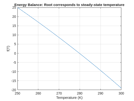
The fzero function can handle extremely messy equations — even those mixing exponentials, trigonometric, and logarithmic terms — provided the function is continuous near the root and you give a reasonable starting point or interval.
It’s ideal for cases like:
- Solving energy balance equations
- Finding intersection points of nonlinear models
- Determining parameters from experimental data
Example: Solving for Equilibrium Temperature in a Heat Radiation-Conduction Model
Suppose a spacecraft component exchanges heat via conduction and radiation with its environment. At steady state, the power generated internally equals the heat lost:
Given constants:
 = 25 W
- k = 0.5 W/K
- ϵ = 0.8
- σ = 5.67e−8 W/m²K⁴
- A = 0.1 m²
 = 250 K
Find the steady-state temperature, T.
% Given constants
Qgen = 25;
k = 0.5;
eps = 0.8;
sigma = 5.67e-8;
A = 0.1;
Tinf = 250;
% Define the energy balance equation (set equal to zero)
f = @(T) Qgen - (k*(T - Tinf) + eps*sigma*A*(T.^4 - Tinf^4));
% Plot for a sense of where the root lies before implementing
fplot(f, [250 300]); grid on
xlabel('Temperature (K)'); ylabel('f(T)')
title('Energy Balance: Root corresponds to steady-state temperature')
% Use fzero with an interval that brackets the root
T_eq = fzero(f, [250 300]);
fprintf('Steady-state temperature: %.2f K\n', T_eq);

It’s exciting to dive into a new dataset full of unfamiliar variables but it can also be overwhelming if you’re not sure where to start. Recently, I discovered some new interactive features in MATLAB live scripts that make it much easier to get an overview of your data. With just a few clicks, you can display sparklines and summary statistics using table variables, sort and filter variables, and even have MATLAB generate the corresponding code for reproducibility.
The Graphics and App Building blog published an article that walks through these features showing how to explore, clean, and analyze data—all without writing any code.
If you’re interested in streamlining your exploratory data analysis or want to see what’s new in live scripts, you might find it helpful:
If you’ve tried these features or have your own tips for quick data exploration in MATLAB, I’d love to hear your thoughts!
Pure Matlab
82%
Simulink
18%
11 votes
I set my 3D matrix up with the players in the 3rd dimension. I set up the matrix with: 1) player does not hold the card (-1), player holds the card (1), and unknown holding the card (0). I moved through the turns (-1 and 1) that are fixed first. Then cycled through the conditional turns (0) while checking the cards of each player using the hints provided until it was solved. The key for me in solving several of the tests (11, 17, and 19) was looking at the 1's and 0's being held by each player.
sum(cardState==1,3);%any zeros in this 2D matrix indicate possible cards in the solution
sum(cardState==0,3)>0;%the ones in this 2D matrix indicate the only unknown positions
sum(cardState==1,3)|sum(cardState==0,3)>0;%oring the two together could provide valuable information
Some MATLAB Cody problems prohibit loops (for, while) or conditionals (if, switch, while), forcing creative solutions.
One elegant trick is to use nested functions and recursion to achieve the same logic — while staying within the rules.
Example: Recursive Summation Without Loops or Conditionals
Suppose loops and conditionals are banned, but you need to compute the sum of numbers from 1 to n. This is a simple example and obvisously n*(n+1)/2 would be preferred.
function s = sumRecursive(n)
zero=@(x)0;
s = helper(n); % call nested recursive function
function out = helper(k)
L={zero,@helper};
out = k+L{(k>0)+1}(k-1);
end
end
sumRecursive(10)
- The helper function calls itself until the base case is reached.
- Logical indexing into a cell array (k>0) act as an 'if' replacement.
- MATLAB allows nested functions to share variables and functions (zero), so you can keep state across calls.
Tips:
- Replace 'if' with logical indexing into a cell array.
- Replace for/while with recursion.
- Nested functions are local and can access outer variables, avoiding global state.
Many MATLAB Cody problems involve recognizing integer sequences.
If a sequence looks familiar but you can’t quite place it, the On-Line Encyclopedia of Integer Sequences (OEIS) can be your best friend.
OEIS will often identify the sequence, provide a formula, recurrence relation, or even direct MATLAB-compatible pseudocode.
Example: Recognizing a Cody Sequence
Suppose you encounter this sequence in a Cody problem:
1, 1, 2, 3, 5, 8, 13, 21, ...
Entering it on OEIS yields A000045 – The Fibonacci Numbers, defined by:
F(n) = F(n-1) + F(n-2), with F(1)=1, F(2)=1
You can then directly implement it in MATLAB:
function F = fibSeq(n)
F = zeros(1,n);
F(1:2) = 1;
for k = 3:n
F(k) = F(k-1) + F(k-2);
end
end
fibSeq(15)
When solving MATLAB Cody problems involving very large integers (e.g., factorials, Fibonacci numbers, or modular arithmetic), you might exceed MATLAB’s built-in numeric limits.
To overcome this, you can use Java’s java.math.BigInteger directly within MATLAB — it’s fast, exact, and often accepted by Cody if you convert the final result to a numeric or string form.
Below is an example of using it to find large factorials.
function s = bigFactorial(n)
import java.math.BigInteger
f = BigInteger('1');
for k = 2:n
f = f.multiply(BigInteger(num2str(k)));
end
s = char(f.toString); % Return as string to avoid overflow
end
bigFactorial(100)
If you have solved a Cody problem before, you have likely seen the Scratch Pad text field below the Solution text field. It provides a quick way to get feedback on your solution before submitting it. Since submitting a solution takes you to a new page, any time a wrong solution is submitted, you have to navigate back to the problem page to try it again.
Instead, I use the Scratch Pad to test my solution repeatedly before submitting. That way, I get to a working solution faster without having to potentially go back and forth many times between the problem page and the wrong-solution page.
Here is my approach:
- Write a tentative solution.
- Copy a test case from the test suite into the Scratch Pad.
- Click the Run Function button—this is immediately below the Scratch Pad and above the Output panel and Submit buttons.
- If the solution does not work, modify the solution code, sometimes putting in disp() lines and/or removing semicolons to trace what the code is doing. Repeat until the solution passes.
- If the solution does work, repeat steps 2 through 4.
- Once there are no more test cases to copy and paste, clean up the code, if necessary (delete disp lines, reinstate all semicolons to suppress output). Click the Run Function button once more, just to make sure I did not break the solution while cleaning it up. Then, click the Submit button.
For problems with large test suites, you may find it useful to copy and paste in multiple test cases per iteration.
Hopefully you find this useful.
Title: Looking for Internship Guidance as a Beginner MATLAB/Simulink Learner
Hello everyone,
I’m a Computer Science undergraduate currently building a strong foundation in MATLAB and Simulink. I’m still at a beginner level, but I’m actively learning every day and can work confidently once I understand the concepts. Right now I’m focusing on MATLAB modeling, physics simulation, and basic control systems so that I can contribute effectively to my current project.
I’m part of an Autonomous Underwater Vehicle (AUV) team preparing for the Singapore AUV Challenge (SAUVC). My role is in physics simulation, controls, and navigation, and MATLAB/Simulink plays a major role in that pipeline. I enjoy physics and mathematics deeply, which makes learning modeling and simulation very exciting for me.
On the coding side, I practice competitive programming regularly—
• Codeforces rating: ~1200
• LeetCode rating: ~1500
So I'm comfortable with logic-building and problem solving. What I’m looking for:
I want to know how a beginner like me can start applying for internships related to MATLAB, Simulink, modeling, simulation, or any engineering team where MATLAB is widely used (including companies outside MathWorks).
I would really appreciate advice from the community on:
- What skills should I strengthen first?
- Which MATLAB/Simulink toolboxes are most important for beginners aiming toward simulation/control roles?
- What small projects or portfolio examples should I build to improve my profile?
- What is the best roadmap to eventually become a good candidate for internships in this area?
Any guidance, resources, or suggestions would be extremely helpful for me.
Thank you in advance to everyone who shares their experience!
Jorge Bernal-AlvizJorge Bernal-Alviz shared the following code that requires R2025a or later:
Test()

function Test()
duration = 10;
numFrames = 800;
frameInterval = duration / numFrames;
w = 400;
t = 0;
i_vals = 1:10000;
x_vals = i_vals;
y_vals = i_vals / 235;
r = linspace(0, 1, 300)';
g = linspace(0, 0.1, 300)';
b = linspace(1, 0, 300)';
r = r * 0.8 + 0.1;
g = g * 0.6 + 0.1;
b = b * 0.9 + 0.1;
customColormap = [r, g, b];
figure('Position', [100, 100, w, w], 'Color', [0, 0, 0]);
axis equal;
axis off;
xlim([0, w]);
ylim([0, w]);
hold on;
colormap default;
colormap(customColormap);
plothandle = scatter([], [], 1, 'filled', 'MarkerFaceAlpha', 0.12);
for i = 1:numFrames
t = t + pi/240;
k = (4 + 3 * sin(y_vals * 2 - t)) .* cos(x_vals / 29);
e = y_vals / 8 - 13;
d = sqrt(k.^2 + e.^2);
c = d - t;
q = 3 * sin(2 * k) + 0.3 ./ (k + 1e-10) + ...
sin(y_vals / 25) .* k .* (9 + 4 * sin(9 * e - 3 * d + 2 * t));
points_x = q + 30 * cos(c) + 200;
points_y = q .* sin(c) + 39 * d - 220;
points_y = w - points_y;
CData = (1 + sin(0.1 * (d - t))) / 3;
CData = max(0, min(1, CData));
set(plothandle, 'XData', points_x, 'YData', points_y, 'CData', CData);
brightness = 0.5 + 0.3 * sin(t * 0.2);
set(plothandle, 'MarkerFaceAlpha', brightness);
drawnow;
pause(frameInterval);
end
end
Parallel Computing Onramp is here! This free, one-hour self-paced course teaches the basics of running MATLAB code in parallel using multiple CPU cores, helping users speed up their code and write code that handles information efficiently.
Remember, Onramps are free for everyone - give the new course a try if you're curious. Let us know what you think of it by replying below.