Results for
In a recent blog post, @Guy Rouleau writes about the new Simulink Copilot Beta. Sign ups are on the Copilot Beta page below. Let him know what you think.
Guy's Blog Post - https://blogs.mathworks.com/simulink/2025/12/01/a-copilot-for-simulink/
Simulink Copilot Beta - https://www.mathworks.com/products/simulink-copilot.html

% Recreation of Saturn photo
figure('Color', 'k', 'Position', [100, 100, 800, 800]);
ax = axes('Color', 'k', 'XColor', 'none', 'YColor', 'none', 'ZColor', 'none');
hold on;
% Create the planet sphere
[x, y, z] = sphere(150);
% Saturn colors - pale yellow/cream gradient
saturn_radius = 1;
% Create color data based on latitude for gradient effect
lat = asin(z);
color_data = rescale(lat, 0.3, 0.9);
% Plot Saturn with smooth shading
planet = surf(x*saturn_radius, y*saturn_radius, z*saturn_radius, ...
color_data, ...
'EdgeColor', 'none', ...
'FaceColor', 'interp', ...
'FaceLighting', 'gouraud', ...
'AmbientStrength', 0.3, ...
'DiffuseStrength', 0.6, ...
'SpecularStrength', 0.1);
% Use a cream/pale yellow colormap for Saturn
cream_map = [linspace(0.4, 0.95, 256)', ...
linspace(0.35, 0.9, 256)', ...
linspace(0.2, 0.7, 256)'];
colormap(cream_map);
% Create the ring system
n_points = 300;
theta = linspace(0, 2*pi, n_points);
% Define ring structure (inner radius, outer radius, brightness)
rings = [
1.2, 1.4, 0.7; % Inner ring
1.45, 1.65, 0.8; % A ring
1.7, 1.85, 0.5; % Cassini division (darker)
1.9, 2.3, 0.9; % B ring (brightest)
2.35, 2.5, 0.6; % C ring
2.55, 2.8, 0.4; % Outer rings (fainter)
];
% Create rings as patches
for i = 1:size(rings, 1)
r_inner = rings(i, 1);
r_outer = rings(i, 2);
brightness = rings(i, 3);
% Create ring coordinates
x_inner = r_inner * cos(theta);
y_inner = r_inner * sin(theta);
x_outer = r_outer * cos(theta);
y_outer = r_outer * sin(theta);
% Front side of rings
ring_x = [x_inner, fliplr(x_outer)];
ring_y = [y_inner, fliplr(y_outer)];
ring_z = zeros(size(ring_x));
% Color based on brightness
ring_color = brightness * [0.9, 0.85, 0.7];
fill3(ring_x, ring_y, ring_z, ring_color, ...
'EdgeColor', 'none', ...
'FaceAlpha', 0.7, ...
'FaceLighting', 'gouraud', ...
'AmbientStrength', 0.5);
end
% Add some texture/gaps in the rings using scatter
n_particles = 3000;
r_particles = 1.2 + rand(1, n_particles) * 1.6;
theta_particles = rand(1, n_particles) * 2 * pi;
x_particles = r_particles .* cos(theta_particles);
y_particles = r_particles .* sin(theta_particles);
z_particles = (rand(1, n_particles) - 0.5) * 0.02;
% Vary particle brightness
particle_colors = repmat([0.8, 0.75, 0.6], n_particles, 1) .* ...
(0.5 + 0.5*rand(n_particles, 1));
scatter3(x_particles, y_particles, z_particles, 1, particle_colors, ...
'filled', 'MarkerFaceAlpha', 0.3);
% Add dramatic outer halo effect - multiple layers extending far out
n_glow = 20;
for i = 1:n_glow
glow_radius = 1 + i*0.35; % Extend much farther
alpha_val = 0.08 / sqrt(i); % More visible, slower falloff
% Color gradient from cream to blue/purple at outer edges
if i <= 8
glow_color = [0.9, 0.85, 0.7]; % Warm cream/yellow
else
% Gradually shift to cooler colors
mix = (i - 8) / (n_glow - 8);
glow_color = (1-mix)*[0.9, 0.85, 0.7] + mix*[0.6, 0.65, 0.85];
end
surf(x*glow_radius, y*glow_radius, z*glow_radius, ...
ones(size(x)), ...
'EdgeColor', 'none', ...
'FaceColor', glow_color, ...
'FaceAlpha', alpha_val, ...
'FaceLighting', 'none');
end
% Add extensive glow to rings - make it much more dramatic
n_ring_glow = 12;
for i = 1:n_ring_glow
glow_scale = 1 + i*0.15; % Extend farther
alpha_ring = 0.12 / sqrt(i); % More visible
for j = 1:size(rings, 1)
r_inner = rings(j, 1) * glow_scale;
r_outer = rings(j, 2) * glow_scale;
brightness = rings(j, 3) * 0.5 / sqrt(i);
x_inner = r_inner * cos(theta);
y_inner = r_inner * sin(theta);
x_outer = r_outer * cos(theta);
y_outer = r_outer * sin(theta);
ring_x = [x_inner, fliplr(x_outer)];
ring_y = [y_inner, fliplr(y_outer)];
ring_z = zeros(size(ring_x));
% Color gradient for ring glow
if i <= 6
ring_color = brightness * [0.9, 0.85, 0.7];
else
mix = (i - 6) / (n_ring_glow - 6);
ring_color = brightness * ((1-mix)*[0.9, 0.85, 0.7] + mix*[0.65, 0.7, 0.9]);
end
fill3(ring_x, ring_y, ring_z, ring_color, ...
'EdgeColor', 'none', ...
'FaceAlpha', alpha_ring, ...
'FaceLighting', 'none');
end
end
% Add diffuse glow particles for atmospheric effect
n_glow_particles = 8000;
glow_radius_particles = 1.5 + rand(1, n_glow_particles) * 5;
theta_glow = rand(1, n_glow_particles) * 2 * pi;
phi_glow = acos(2*rand(1, n_glow_particles) - 1);
x_glow = glow_radius_particles .* sin(phi_glow) .* cos(theta_glow);
y_glow = glow_radius_particles .* sin(phi_glow) .* sin(theta_glow);
z_glow = glow_radius_particles .* cos(phi_glow);
% Color particles based on distance - cooler colors farther out
particle_glow_colors = zeros(n_glow_particles, 3);
for i = 1:n_glow_particles
dist = glow_radius_particles(i);
if dist < 3
particle_glow_colors(i,:) = [0.9, 0.85, 0.7];
else
mix = (dist - 3) / 4;
particle_glow_colors(i,:) = (1-mix)*[0.9, 0.85, 0.7] + mix*[0.5, 0.6, 0.9];
end
end
scatter3(x_glow, y_glow, z_glow, rand(1, n_glow_particles)*2+0.5, ...
particle_glow_colors, 'filled', 'MarkerFaceAlpha', 0.05);
% Lighting setup
light('Position', [-3, -2, 4], 'Style', 'infinite', ...
'Color', [1, 1, 0.95]);
light('Position', [2, 3, 2], 'Style', 'infinite', ...
'Color', [0.3, 0.3, 0.4]);
% Camera and view settings
axis equal off;
view([-35, 25]); % Angle to match saturn_photo.jpg - more dramatic tilt
camva(10); % Field of view - slightly wider to show full halo
xlim([-8, 8]); % Expanded to show outer halo
ylim([-8, 8]);
zlim([-8, 8]);
% Material properties
material dull;
title('Saturn - Left click: Rotate | Right click: Pan | Scroll: Zoom', 'Color', 'w', 'FontSize', 12);
% Enable interactive camera controls
cameratoolbar('Show');
cameratoolbar('SetMode', 'orbit'); % Start in rotation mode

% Custom mouse controls
set(gcf, 'WindowButtonDownFcn', @mouseDown);
function mouseDown(src, ~)
selType = get(src, 'SelectionType');
switch selType
case 'normal' % Left click - rotate
cameratoolbar('SetMode', 'orbit');
rotate3d on;
case 'alt' % Right click - pan
cameratoolbar('SetMode', 'pan');
pan on;
end
end
Experimenting with Agentic AI
44%
I am an AI skeptic
0%
AI is banned at work
11%
I am happy with Conversational AI
44%
9 votes
Run MATLAB using AI applications by leveraging MCP. This MCP server for MATLAB supports a wide range of coding agents like Claude Code and Visual Studio Code.
Check it out and share your experiences below. Have fun!
GitHub repo: https://github.com/matlab/matlab-mcp-core-server
Yann Debray's blog post: https://blogs.mathworks.com/deep-learning/2025/11/03/releasing-the-matlab-mcp-core-server-on-github/
Pick a team, solve Cody problems, and share your best tips and tricks. Whether you’re a beginner or a seasoned MATLAB user, you’ll have fun learning, connecting with others, and competing for amazing prizes, including MathWorks swags, Amazon gift cards, and virtual badges.
How to Participate
- Join a team that matches your coding personality
- Solve Cody problems, complete the contest problem group, or share Tips & Tricks articles
- Bonus Round: Two top players from each team will be invited to a fun code-along event
Contest Timeline
- Main Round: Nov 10 – Dec 7, 2025
- Bonus Round: Dec 8 – Dec 19, 2025
Prizes (updated 11/19)
- (New prize) Solving just one problem in the contest problem group gives you a chance to win MathWorks T-shirts or socks each week.
- Finishing the entire problem group will greatly increase your chances—while helping your team win.
- Share high-quality Tips & Tricks articles to earn you a coveted MathWorks Yeti Bottle.
- Become a top finisher in your team to win Amazon gift cards and an invitation to the bonus round.
Automating Parameter Identifiability Analysis in SimBiology
Is it possible to develop a MATLAB Live Script that automates a series of SimBiology model fits to obtain likelihood profiles? The goal is to fit a kinetic model to experimental data while systematically fixing the value of one kinetic constant (e.g., k1) and leaving the others unrestricted.
The script would perform the following:
Use a pre-configured SimBiology project where the best fit to the experimental data has already been established (including dependent/independent variables, covariates, the error model, and optimization settings).
Iterate over a defined sequence of fixed values for a chosen parameter.
For each fixed value, run the estimation to optimize the remaining parameters.
Record the resulting Sum of Squared Errors (SSE) for each run.
The final output would be a likelihood profile—a plot of SSE versus the fixed parameter value (e.g., k1)—to assess the practical identifiability of each model parameter.
For the www, uk, and in domains,a generative search answer is available for Help Center searches. Please let us know if you get good or bad results for your searches. Some have pointed out that it is not available in non-english domains. You can switch your country setting to try it out. You can also ask questions in different languages and ask for the response in a different language. I get better results when I ask more specific queries. How is it working for you?
Hello MATLAB Central community,
My name is Yann. And I love MATLAB. I also love Python ... 🐍 (I know, not the place for that).
I recently decided to go down the rabbit hole of AI. So I started benchmarking deep learning frameworks on basic examples. Here is a recording of my experiment:
Happy to engage in the debate. What do you think?
Large Language Models (LLMs) with MATLAB was updated again today to support the newly released OpenAI models GPT-5, GPT-5 mini, GPT-5 nano, GPT-5 chat, o3, and o4-mini. When you create an openAIChat object, set the ModelName name-value argument to "gpt-5", "gpt-5-mini", "gpt-5-nano", "gpt-5-chat-latest", "o4-mini", or "o3".
This is version 4.4.0 of this free MATLAB add-on that lets you interact with LLMs on MATLAB. The release notes are at Release v4.4.0: Support for GPT-5, o3, o4-mini · matlab-deep-learning/llms-with-matlab
Hi everyone,
Please check out our new book "Generative AI for Trading and Asset Management".
GenAI is usually associated with large language models (LLMs) like ChatGPT, or with image generation tools like MidJourney, essentially, machines that can learn from text or images and generate text or images. But in reality, these models can learn from many different types of data. In particular, they can learn from time series of asset returns, which is perhaps the most relevant for asset managers.
In our book (amazon.com link), we explore both the practical applications and the fundamental principles of GenAI, with a special focus on how these technologies apply to trading and asset management.
The book is divided into two broad parts:
Part 1 is written by Ernie Chan, noted author of Quantitative Trading, Algorithmic Trading, and Machine Trading. It starts with no-code applications of GenAI for traders and asset managers with little or no coding experience. After that, it takes readers on a whirlwind tour of machine learning techniques commonly used in finance.
Part 2, written by Hamlet, covers the fundamentals and technical details of GenAI, from modeling to efficient inference. This part is for those who want to understand the inner workings of these models and how to adapt them to their own custom data and applications. It’s for anyone who wants to go beyond the high-level use cases, get their hands dirty, and apply, and eventually improve these models in real-world practical applications.
Readers can start with whichever part they want to explore and learn from.
I am deeply honored to announce the official publication of my latest academic volume:
MATLAB for Civil Engineers: From Basics to Advanced Applications
(Springer Nature, 2025).
This work serves as a comprehensive bridge between theoretical civil engineering principles and their practical implementation through MATLAB—a platform essential to the future of computational design, simulation, and optimization in our field.
Structured to serve both academic audiences and practicing engineers, this book progresses from foundational MATLAB programming concepts to highly specialized applications in structural analysis, geotechnical engineering, hydraulic modeling, and finite element methods. Whether you are a student building analytical fluency or a professional seeking computational precision, this volume offers an indispensable resource for mastering MATLAB's full potential in civil engineering contexts.
With rigorously structured examples, case studies, and research-aligned methods, MATLAB for Civil Engineers reflects the convergence of engineering logic with algorithmic innovation—equipping readers to address contemporary challenges with clarity, accuracy, and foresight.
📖 Ideal for:
— Graduate and postgraduate civil engineering students
— University instructors and lecturers seeking a structured teaching companion
— Professionals aiming to integrate MATLAB into complex real-world projects
If you are passionate about engineering resilience, data-informed design, or computational modeling, I invite you to explore the work and share it with your network.
🧠 Let us advance the discipline together through precision, programming, and purpose.
The Graphics and App Building Blog just launched its first article on R2025a features, authored by Chris Portal, the director of engineering for the MATLAB graphics and app building teams.
Over the next few months, we'll publish a series of articles that showcase our updated graphics system, introduce new tools and features, and provide valuable references enriched by the perspectives of those involved in their development.
To stay updated, you can subscribe to the blog (look for the option in the upper left corner of the blog page). We also encourage you to join the conversation—your comments and questions under each article help shape the discussion and guide future content.
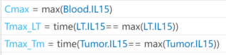
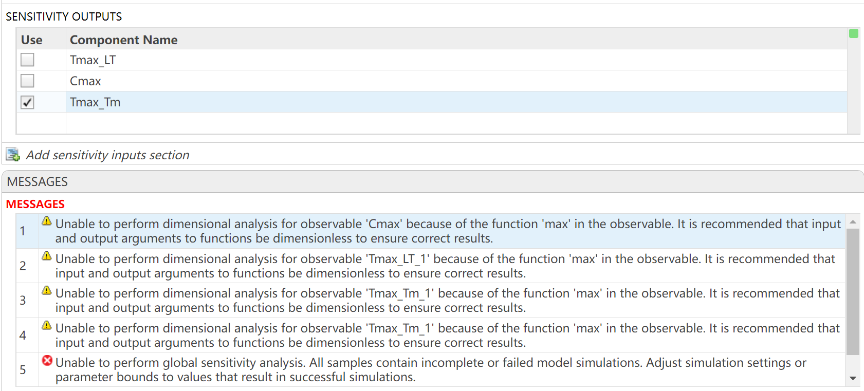
I want to observe the time (Tmax) to reach maximum drug concentration (Cmax) in my model. I have set up the OBSERVABLES as follows (figure1): Cmax = max(Blood.lL15); Tmax_LT = time(Conc_lL15_LT_nm == max(Conc_lL15_LT_nm)); Tmax_Tm = time(Conc_lL15_Tumor_nm == max(Conc_lL15_Tumor_nm)); After running the Sobol indices program for global sensitivity analysis, with inputs being some parameters and their ranges, the output for Cmax works, but there are some prompts, as shown in figure2. Additionally, when outputting Tmax, the program does not run successfully and reports some errors, as shown in figure2. How can I resolve the errors when outputting Tmax?
Large Languge model with MATLAB, a free add-on that lets you access LLMs from OpenAI, Azure, amd Ollama (to use local models) on MATLAB, has been updated to support OpenAI GPT-4.1, GPT-4.1 mini, and GPT-4.1 nano.
According to OpenAI, "These models outperform GPT‑4o and GPT‑4o mini across the board, with major gains in coding and instruction following. They also have larger context windows—supporting up to 1 million tokens of context—and are able to better use that context with improved long-context comprehension."
What would you build with the latest update?

Provide insightful answers
9%
Provide label-AI answer
9%
Provide answer by both AI and human
21%
Do not use AI for answers
46%
Give a button "chat with copilot"
10%
use AI to draft better qustions
5%
1561 votes
%% 清理环境
close all; clear; clc;
%% 模拟时间序列
t = linspace(0,12,200); % 时间从 0 到 12,分 200 个点
% 下面构造一些模拟的"峰状"数据,用于演示
% 你可以根据需要替换成自己的真实数据
rng(0); % 固定随机种子,方便复现
baseIntensity = -20; % 强度基线(z 轴的最低值)
numSamples = 5; % 样本数量
yOffsets = linspace(20,140,numSamples); % 不同样本在 y 轴上的偏移
colors = [ ...
0.8 0.2 0.2; % 红
0.2 0.8 0.2; % 绿
0.2 0.2 0.8; % 蓝
0.9 0.7 0.2; % 金黄
0.6 0.4 0.7]; % 紫
% 构造一些带多个峰的模拟数据
dataMatrix = zeros(numSamples, length(t));
for i = 1:numSamples
% 随机峰参数
peakPositions = randperm(length(t),3); % 三个峰位置
intensities = zeros(size(t));
for pk = 1:3
center = peakPositions(pk);
width = 10 + 10*rand; % 峰宽
height = 100 + 50*rand; % 峰高
% 高斯峰
intensities = intensities + height*exp(-((1:length(t))-center).^2/(2*width^2));
end
% 再加一些小随机扰动
intensities = intensities + 10*randn(size(t));
dataMatrix(i,:) = intensities;
end
%% 开始绘图
figure('Color','w','Position',[100 100 800 600],'Theme','light');
hold on; box on; grid on;
for i = 1:numSamples
% 构造 fill3 的多边形顶点
xPatch = [t, fliplr(t)];
yPatch = [yOffsets(i)*ones(size(t)), fliplr(yOffsets(i)*ones(size(t)))];
zPatch = [dataMatrix(i,:), baseIntensity*ones(size(t))];
% 使用 fill3 填充面积
hFill = fill3(xPatch, yPatch, zPatch, colors(i,:));
set(hFill,'FaceAlpha',0.8,'EdgeColor','none'); % 调整透明度、去除边框
% 在每条曲线尾部标注 Sample i
text(t(end)+0.3, yOffsets(i), dataMatrix(i,end), ...
['Sample ' num2str(i)], 'FontSize',10, ...
'HorizontalAlignment','left','VerticalAlignment','middle');
end
%% 坐标轴与视角设置
xlim([0 12]);
ylim([0 160]);
zlim([-20 350]);
xlabel('Time (sec)','FontWeight','bold');
ylabel('Frequency (Hz)','FontWeight','bold');
zlabel('Intensity','FontWeight','bold');
% 设置刻度(根据需要微调)
set(gca,'XTick',0:2:12, ...
'YTick',0:40:160, ...
'ZTick',-20:40:200);
% 设置视角(az = 水平旋转,el = 垂直旋转)
view([211 21]);
% 让三维坐标轴在后方
set(gca,'Projection','perspective');
% 如果想去掉默认的坐标轴线,也可以尝试
% set(gca,'BoxStyle','full','LineWidth',1.2);
%% 可选:在后方添加一个浅色网格平面 (示例)
% 这个与题图右上方的网格类似
[Xplane,Yplane] = meshgrid([0 12],[0 160]);
Zplane = baseIntensity*ones(size(Xplane)); % 在 Z = -20 处画一个竖直面的框
surf(Xplane, Yplane, Zplane, ...
'FaceColor',[0.95 0.95 0.9], ...
'EdgeColor','k','FaceAlpha',0.3);
%% 进一步美化(可根据需求调整)
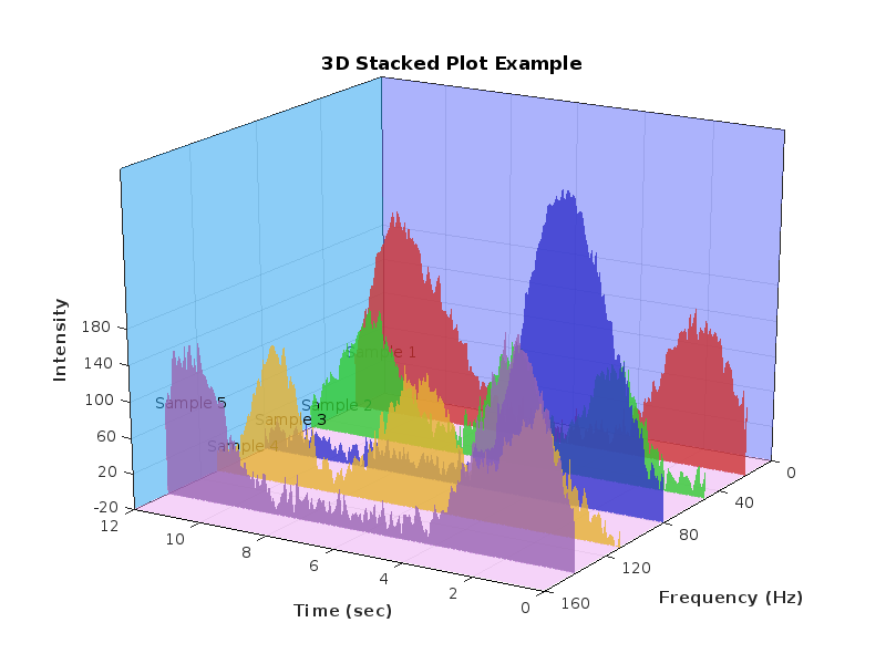
title('3D Stacked Plot Example','FontSize',12);
constantplane("x",12,FaceColor=rand(1,3),FaceAlpha=0.5);
constantplane("y",0,FaceColor=rand(1,3),FaceAlpha=0.5);
constantplane("z",-19,FaceColor=rand(1,3),FaceAlpha=0.5);
hold off;
Have fun! Enjoy yourself!
Hello Community,
We're excited to announce that registration is now open for the MathWorks AUTOMOTIVE CONFERENCE 2025! This event presents a fantastic opportunity to connect with MathWorks and industry experts while exploring the latest trends in the automotive sector.
Event Details:
- Date: April 29, 2025
- Location: St. John’s Resort, Plymouth, MI
Featured Topics:
- Virtual Development
- Electrification
- Software Development
- AI in Engineering
Whether you're a professional in the automotive industry or simply interested in these cutting-edge topics, we highly encourage you to register for this conference.
We look forward to seeing you there!
We are excited to announce another update to our Discussions area: the new Contribution Widget! The new widget simplifies the process of creating diverse types of content, whether you're praising someone who has helped you, sharing tips and tricks, or polling the community.

Previously, creating various types of content required navigating multiple links or channels. With the new Contribution Widget, everything you need is conveniently located in one place.
Give it a try and let us know how we can further enhance your user experience.
P.S. Who has been particularly helpful to you lately? Create your first praise post and let them know!
We are excited to announce the first edition of the MathWorks AI Challenge. You’re invited to submit innovative solutions to challenges in the field of artificial intelligence. Choose a project from our curated list and submit your solution for a chance to win up to $1,000 (USD). Showcase your creativity and contribute to the advancement of AI technology.
I am pleased to announce the 6th Edition of my book MATLAB Recipes for Earth Sciences with Springer Nature
also in the MathWorks Book Program
It is now almost exactly 20 years since I signed the contract with Springer for the first edition of the book. Since then, the book has grown from 237 to 576 pages, with many new chapters added. I would like to thank my colleagues Norbert Marwan and Robin Gebbers, who have each contributed two sections to Chapters 5, 7 and 9.
And of course, my thanks go to the excellent team at the MathWorks Book Program and the numerous other MathWorks experts who have helped and advised me during the last 30+ years working with MATLAB. And of course, thank you Springer for 20 years of support.
This book introduces methods of data analysis in the earth sciences using MATLAB, such as basic statistics for univariate, bivariate, and multivariate data sets, time series analysis, signal processing, spatial and directional data analysis, and image analysis.
Martin H. Trauth