Results for
My thingSpeak channel kept on updateing the same signal as early eventhough my simulink have update the new signal. How to solve this?
Any one have deep learning reinforcement based speed control of induction motor?
Hi ThingSpeak Community,
I hope you are all doing well.
I am currently setting up a Vodafone ACL for a SIM card that will be used in a device destined for a remote charity deployment in a week. The goal is to ensure that the device can reliably upload data to ThingSpeak without any connectivity issues.
Here are the details of my current ACL setup:
- FQDN: api.thingspeak.com (specified as the API endpoint)
- IPv4 Address: 184.106.153.149 (found online)
- Port: (left empty)
I've attached a photo of the setup for reference.
Could you please confirm if the above ACL settings are correct? Additionally, if there are any other considerations or settings I should be aware of for ensuring reliable connectivity with ThingSpeak, I would greatly appreciate your guidance.
Currently, all I am using for the device credentials is the PIN number. Do I need to adjust any settings in the Arduino code or the ACL to maintain stable connectivity with ThingSpeak, especially considering the device will be in a remote location and difficult to access for adjustments?
Your prompt assistance and advice will be immensely valuable, as I want to ensure everything is correctly configured before deployment.
Thank you very much!
Best regards,
Arthur
An option for 10th degree polynomials but no weighted linear least squares. Seriously? Jesse
What do you think about the NVIDIA's achivement of becoming the top giant of manufacturing chips, especially for AI world?

错误使用 ipqpdense
The interior convex algorithm requires all objective and constraint values to be finite.
出错 quadprog
ipqpdense(full(H), f, A, B, Aeq, Beq, lb, ub, X0, flags, ...
出错 MPC_maikenamulun
[X, fval,exitflag]=quadprog(H,f,A_cons,B_cons,[],[],lb,ub,[],options);
Hi to everyone!
To simplify the explanation and the problem, I simulated the kinetics of an irreversible first-order reaction, A -> B. I implemented it in two independent compartments, R and P. I simulated the effect of a dilution in R by doubling at t= 0,1 the R volume. I programmed in P that, at t = 0.1, the instantaneous concentration of A and B would be reduced by half. I am sending an attach with the implementation of these simulations in the Simbiology interface.
When the simulations of the two compartments are plotted, it can be seen that the responses are not equal. That is, from t = 0.1 s, the reaction follow an exponential function in R with half of the initial amplitude and half of the initial value of k1. That is, the relaxation time is doubled. Meanwhile, in P, from t = 0.1, the reaction follows exponential kinetics with half the amplitude value but maintaining the initial value of k = 10. Without a doubt, the correct simulation is the latter (compartment P) where only the effect is observed in the amplitude and not in the relaxation time. Could you tell me what the error is that makes these kinetics that should be equal not be?
Thank you in advance!
Luis B.
Hi All,
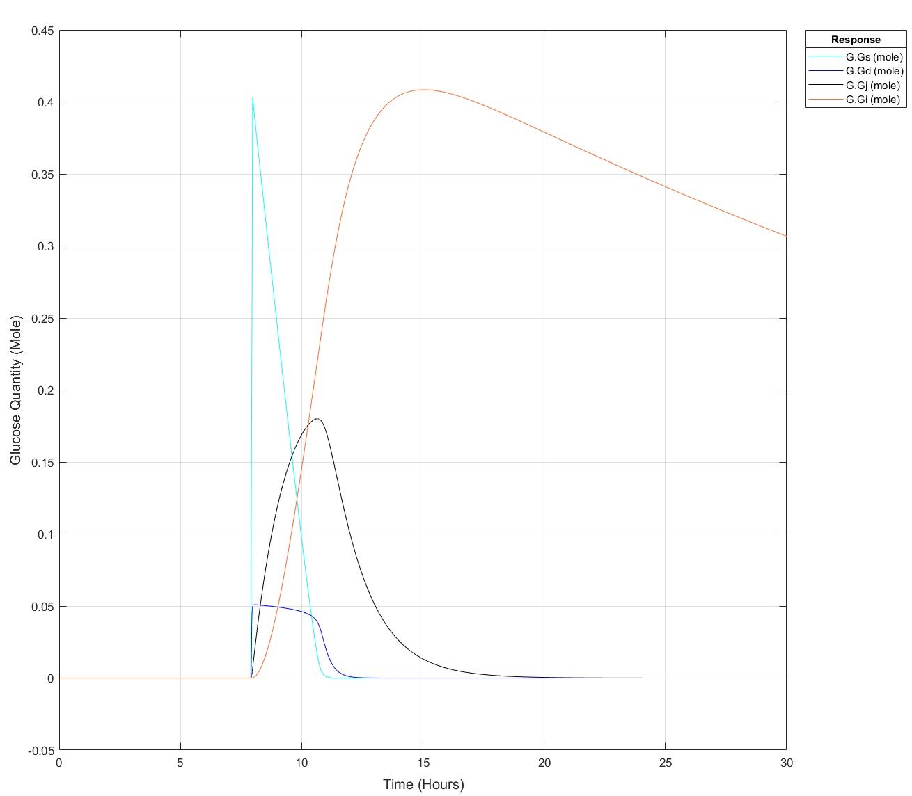
I've been producing a QSP model of glucose homeostasis for a while now for my PhD project, recently I've been able to expand it to larger time series, i.e. 2 days of data rather than a singular injection or a singular meal. My problem is as follows: If I put 75g of glucose into my stomach glucose species any later than (exactly) 8.5 hours I get an integration tolerance error. Curiosly, I can put 25g of glucose in at any time up to 15.9 hours, then any later an error. I have disabled all connections to my glucose absorption chain, i.e. stomach -> duodenum -> jenenum -> ileum -> removal, to isolate the cause of this. I had initially thought it may be because I mechanistically model liver glycogen and that does deplete over time, but I've tested enough to show that that does nothing. My next test is to isolate the glucose absorption chain into a seperate model and see if the issue persists but I'm completely baffled!
These are the equations, to my eye there's no reason why there would be such a sharp glucose quantity/time dependence, they all begin at a value of 0:
d(Gs)/dt = -(kw*(1-Gd^14/(Igd^14+Gd^14))*Gs) #Stomach glucose
d(Gd)/dt = (kw*(1-Gd^14/(Igd^14+Gd^14))*Gs) - (kdj*Gd) #Duodenal Glucose
d(Gj)/dt = (kdj*Gd) - (kji*Gj) #Jejunal Glucose
d(Gi)/dt = (kji*Gj) - (kic*Gi) #Ileal Glucose
(The sigmoidicity of gastric emptying slowing term (^14) was parameterised off of paracetamol absorption data and appears to be correct!)
Thank you for your help, best regards,
Dan
Pre-Edit: I changed the run time to 30 hours and now I can't use the 75g input any later than 7.9 hours not 8.5 hours anymore!
Edit: This is how it appears at all times prior to it failing for 75g:
I have lon and lat and signal stengths plotting from my roaming GPS Lora module that reports signal strength to Thingspeak at it's location. I got GEOSCATTER plotting location circles.But i want extrapulate?Interp?Heatmap. the stengths between the points. When i use Interp i end up timiming out. How do i modify my code to do this?
Public Channel 214526
Cheers Andy
The study of the dynamics of the discrete Klein - Gordon equation (DKG) with friction is given by the equation :

In the above equation, W describes the potential function: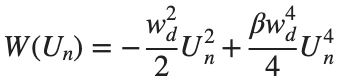
to which every coupled unit  adheres. In Eq. (1), the variable $
 $ is the unknown displacement of the oscillator occupying the n-th position of the lattice, and
  is the discretization parameter. We denote by h the distance between the oscillators of the lattice. The chain (DKG) contains linear damping with a damping coefficient
  , while
 is the coefficient of the nonlinear cubic term.
$ is the unknown displacement of the oscillator occupying the n-th position of the lattice, and For the DKG chain (1), we will consider the problem of initial-boundary values, with initial conditions

and Dirichlet boundary conditions at the boundary points  and
and  , that is,
and , that is,
Therefore, when necessary, we will use the short notation  for the one-dimensional discrete Laplacian
for the one-dimensional discrete Laplacian
Now we want to investigate numerically the dynamics of the system (1)-(2)-(3). Our first aim is to conduct a numerical study of the property of Dynamic Stability of the system, which directly depends on the existence and linear stability of the branches of equilibrium points.
For the discussion of numerical results, it is also important to emphasize the role of the parameter  . By changing the time variable
  , we rewrite Eq. (1) in the form
 . We consider spatially extended initial conditions of the form:
We also assume zero initial velocity:
the following graphs for  and
and 
% Parameters
L = 200; % Length of the system
K = 99; % Number of spatial points
j = 2; % Mode number
omega_d = 1; % Characteristic frequency
beta = 1; % Nonlinearity parameter
delta = 0.05; % Damping coefficient
% Spatial grid
h = L / (K + 1);
n = linspace(-L/2, L/2, K+2); % Spatial points
N = length(n);
omegaDScaled = h * omega_d;
deltaScaled = h * delta;
% Time parameters
dt = 1; % Time step
tmax = 3000; % Maximum time
tspan = 0:dt:tmax; % Time vector
% Values of amplitude 'a' to iterate over
a_values = [2, 1.95, 1.9, 1.85, 1.82]; % Modify this array as needed
% Differential equation solver function
function dYdt = odefun(~, Y, N, h, omegaDScaled, deltaScaled, beta)
U = Y(1:N);
Udot = Y(N+1:end);
Uddot = zeros(size(U));
% Laplacian (discrete second derivative)
for k = 2:N-1
Uddot(k) = (U(k+1) - 2 * U(k) + U(k-1)) ;
end
% System of equations
dUdt = Udot;
dUdotdt = Uddot - deltaScaled * Udot + omegaDScaled^2 * (U - beta * U.^3);
% Pack derivatives
dYdt = [dUdt; dUdotdt];
end
% Create a figure for subplots
figure;
% Initial plot
a_init = 2; % Example initial amplitude for the initial condition plot
U0_init = a_init * sin((j * pi * h * n) / L); % Initial displacement
U0_init(1) = 0; % Boundary condition at n = 0
U0_init(end) = 0; % Boundary condition at n = K+1
subplot(3, 2, 1);
plot(n, U0_init, 'r.-', 'LineWidth', 1.5, 'MarkerSize', 10); % Line and marker plot
xlabel('$x_n$', 'Interpreter', 'latex');
ylabel('$U_n$', 'Interpreter', 'latex');
title('$t=0$', 'Interpreter', 'latex');
set(gca, 'FontSize', 12, 'FontName', 'Times');
xlim([-L/2 L/2]);
ylim([-3 3]);
grid on;
% Loop through each value of 'a' and generate the plot
for i = 1:length(a_values)
a = a_values(i);
% Initial conditions
U0 = a * sin((j * pi * h * n) / L); % Initial displacement
U0(1) = 0; % Boundary condition at n = 0
U0(end) = 0; % Boundary condition at n = K+1
Udot0 = zeros(size(U0)); % Initial velocity
% Pack initial conditions
Y0 = [U0, Udot0];
% Solve ODE
opts = odeset('RelTol', 1e-5, 'AbsTol', 1e-6);
[t, Y] = ode45(@(t, Y) odefun(t, Y, N, h, omegaDScaled, deltaScaled, beta), tspan, Y0, opts);
% Extract solutions
U = Y(:, 1:N);
Udot = Y(:, N+1:end);
% Plot final displacement profile
subplot(3, 2, i+1);
plot(n, U(end,:), 'b.-', 'LineWidth', 1.5, 'MarkerSize', 10); % Line and marker plot
xlabel('$x_n$', 'Interpreter', 'latex');
ylabel('$U_n$', 'Interpreter', 'latex');
title(['$t=3000$, $a=', num2str(a), '$'], 'Interpreter', 'latex');
set(gca, 'FontSize', 12, 'FontName', 'Times');
xlim([-L/2 L/2]);
ylim([-2 2]);
grid on;
end
% Adjust layout
set(gcf, 'Position', [100, 100, 1200, 900]); % Adjust figure size as needed
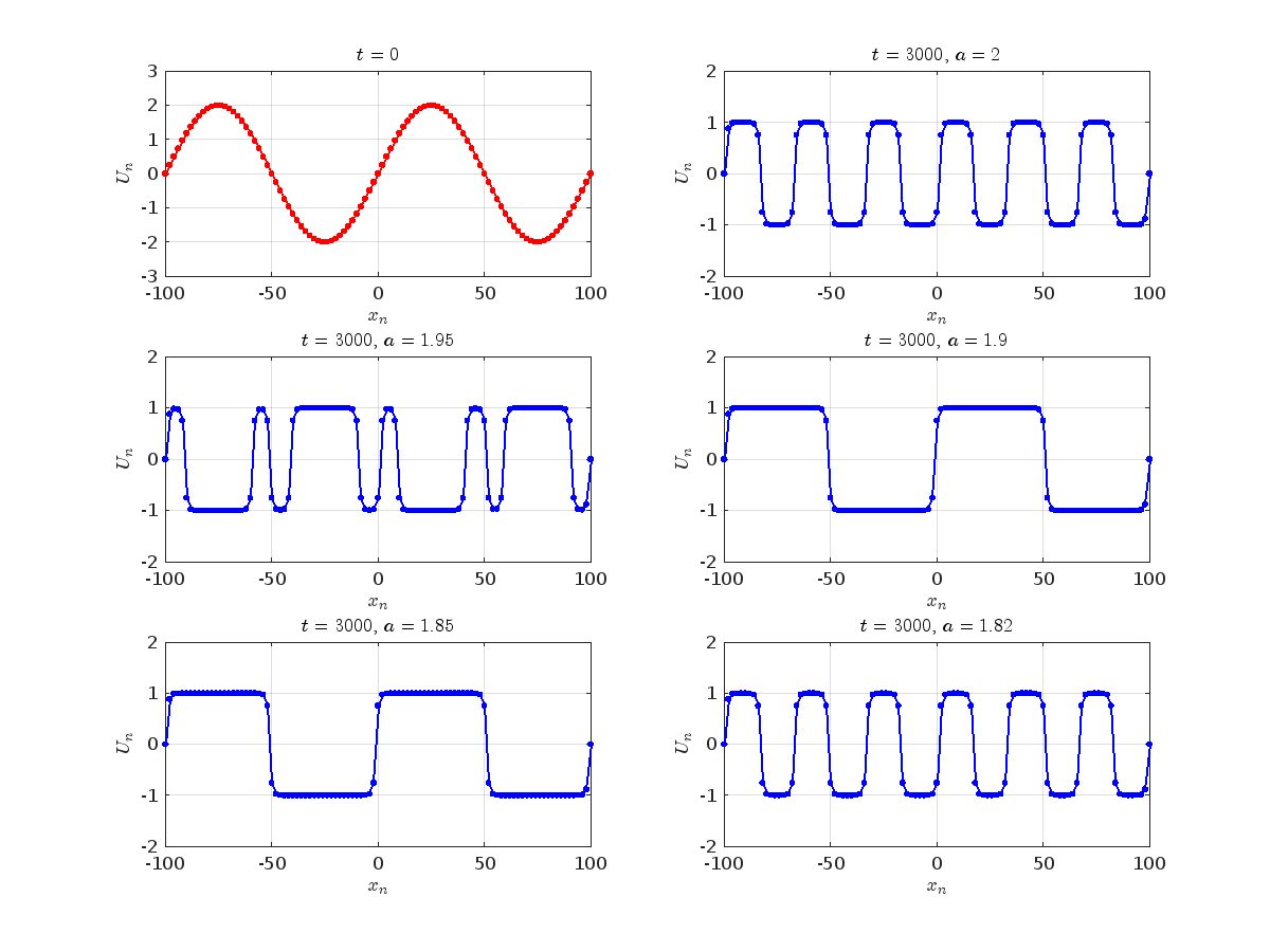
Dynamics for the initial condition ,  , for
, for  , for different amplitude values. By reducing the amplitude values, we observe the convergence to equilibrium points of different branches from
  and the appearance of values
  for which the solution converges to a non-linear equilibrium point
  Parameters:
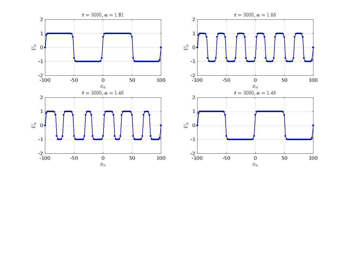
Detection of a stability threshold  : For
: For  , the initial condition ,
  , converges to a non-linear equilibrium point
 .
.
Characteristics for  , with corresponding norm
  where the dynamics appear in the first image of the third row, we observe convergence to a non-linear equilibrium point of branch
  This has the same norm and the same energy as the previous case but the final state has a completely different profile. This result suggests secondary bifurcations have occurred in branch
where the dynamics appear in the first image of the third row, we observe convergence to a non-linear equilibrium point of branch By further reducing the amplitude, distinct values of  are discerned: 1.9, 1.85, 1.81 for which the initial condition
  with norms
  respectively, converges to a non-linear equilibrium point of branch
  This equilibrium point has norm
  and energy
  . The behavior of this equilibrium is illustrated in the third row and in the first image of the third row of Figure 1, and also in the first image of the third row of Figure 2. For all the values between the aforementioned a, the initial condition
  converges to geometrically different non-linear states of branch
  as shown in the second image of the first row and the first image of the second row of Figure 2, for amplitudes
  and
and  respectively.
respectively, converges to a non-linear equilibrium point of branch and energy Refference:
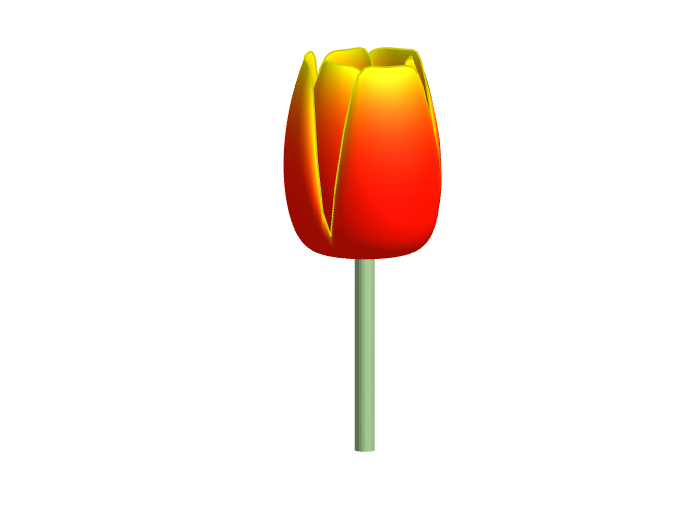
Spring is here in Natick and the tulips are blooming! While tulips appear only briefly here in Massachusetts, they provide a lot of bright and diverse colors and shapes. To celebrate this cheerful flower, here's some code to create your own tulip!
Check out this episode about PIVLab: https://www.buzzsprout.com/2107763/15106425
Join the conversation with William Thielicke, the developer of PIVlab, as he shares insights into the world of particle image velocimetery (PIV) and its applications. Discover how PIV accurately measures fluid velocities, non invasively revolutionising research across the industries. Delve into the development journey of PI lab, including collaborations, key features and future advancements for aerodynamic studies, explore the advanced hardware setups camera technologies, and educational prospects offered by PIVlab, for enhanced fluid velocity measurements. If you are interested in the hardware he speaks of check out the company: Optolution.
One of the starter prompts is about rolling two six-sided dice and plot the results. As a hobby, I create my own board games. I was able to use the dice rolling prompt to show how a simple roll and move game would work. That was a great surprise!
Hallo zusammen,
seit ein paar Tagen werden sämtliche meiner Visualisierungen nicht mehr aktualisiert. Im Editiermodus läuft der Code durch und die Grafik wird korrekt erzeugt.
Hat jemand eine Idee was da schief läuft?
Danke & viele Grüße
Let's talk about probability theory in Matlab.
Conditions of the problem - how many more letters do I need to write to the sales department to get an answer?
To get closer to the problem, I need to buy a license under a contract. Maybe sometimes there are responsible employees sitting here who will give me an answer.
Thank you
In the MATLAB description of the algorithm for Lyapunov exponents, I believe there is ambiguity and misuse.
The lambda(i) in the reference literature signifies the Lyapunov exponent of the entire phase space data after expanding by i time steps, but in the calculation formula provided in the MATLAB help documentation, Y_(i+K) represents the data point at the i-th point in the reconstructed data Y after K steps, and this calculation formula also does not match the calculation code given by MATLAB. I believe there should be some misguidance and misunderstanding here.
According to the symbol regulations in the algorithm description and the MATLAB code, I think the correct formula might be y(i) = 1/dt * 1/N * sum_j( log( ||Y_(j+i) - Y_(j*+i)|| ) )
Cordial saludo , Necesito simular un generador electrico que tiene una entrada mecanica y genera el suficiente voltage y corriente para encender un LED.
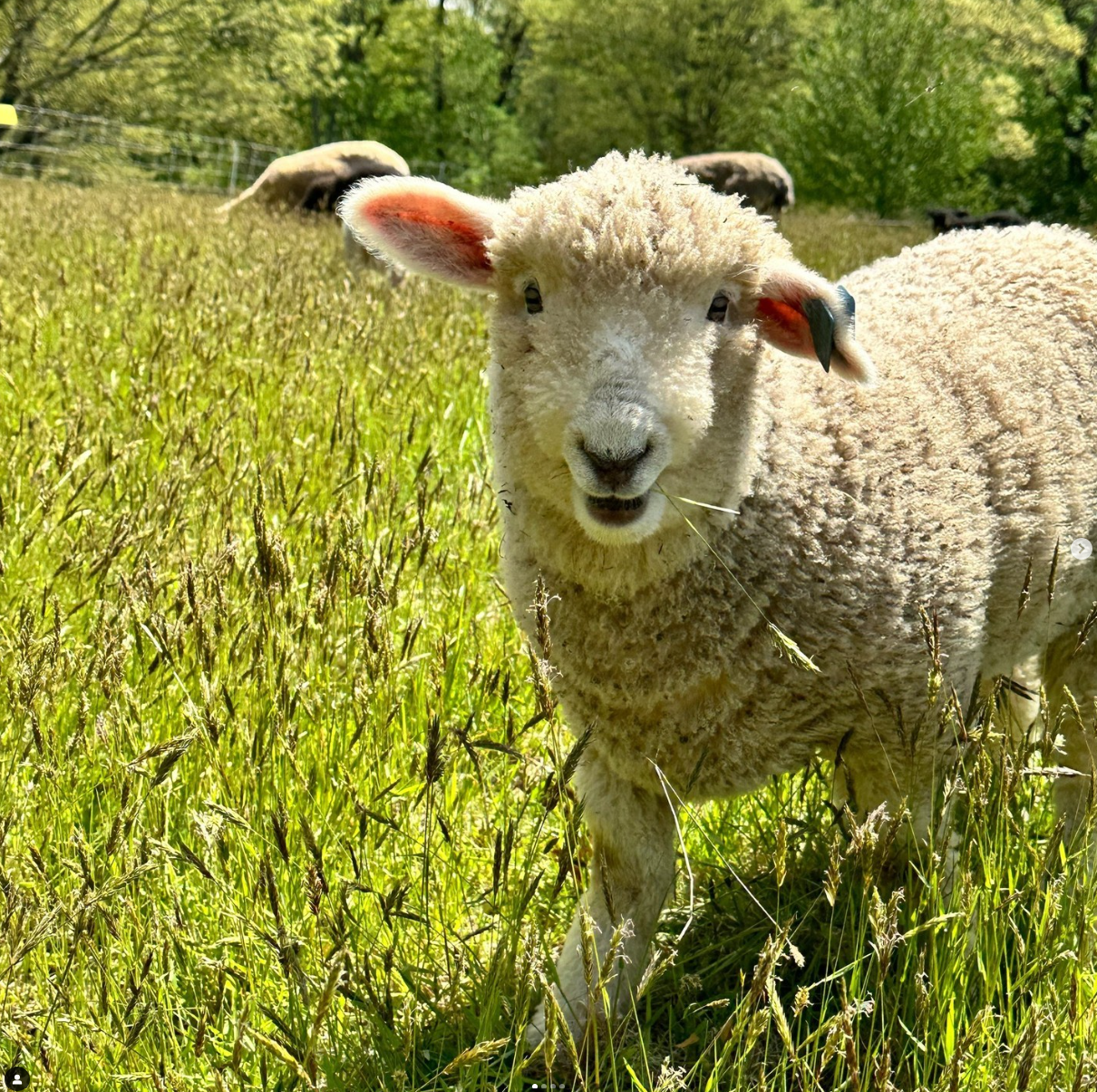
Drumlin Farm has welcomed MATLAMB, named in honor of MathWorks, among ten adorable new lambs this season!
Hi Helpdesk,
I urgently seek assistance with an issue that has persisted for a week. I am using Node-RED to interface my gateway and vibration sensor. The sensor sends 960 packets of X, Y, and Z data every 5 minutes. I retrieve and send this data through my Thingspeak42 node to my Thingspeak channel.
I am subscribed to the Thingspeak Student paid plan (see attached "12.png"). Despite this, Thingspeak is inconsistently snipping my data. For example, my X-field sometimes receives only 78 out of 960 points, and similar inconsistencies occur with the Y and Z fields.
Attached is "vibration data node red.png," showing an attempt to send just 120 packets to my Thingspeak channel. However, only 93 data points are received. Also attached is a JSON snapshot of field 2 - X_values, showing only 93 points ("JSON Field 2 data.png"). This is disappointing given that I am paying for the student plan, which should support 33 million points/year per unit (~90,000/day per unit).
I urgently require an explanation and resolution for this issue. Please provide immediate assistance.
Kind regards,
Krish
I have an Arduino Uno R3 with an integrated ESP 8266. With the Arduino Uno, I measure some capacitive humidity sensors and a DHT 22 temperature and humidity sensor. The measurements are sent to the serial port and the ESP 8266 picks them up and uploads them to ThingSpeak. My problem is that it does this randomly and not in the assigned fields. Could someone help me? Thank you very much