Results for
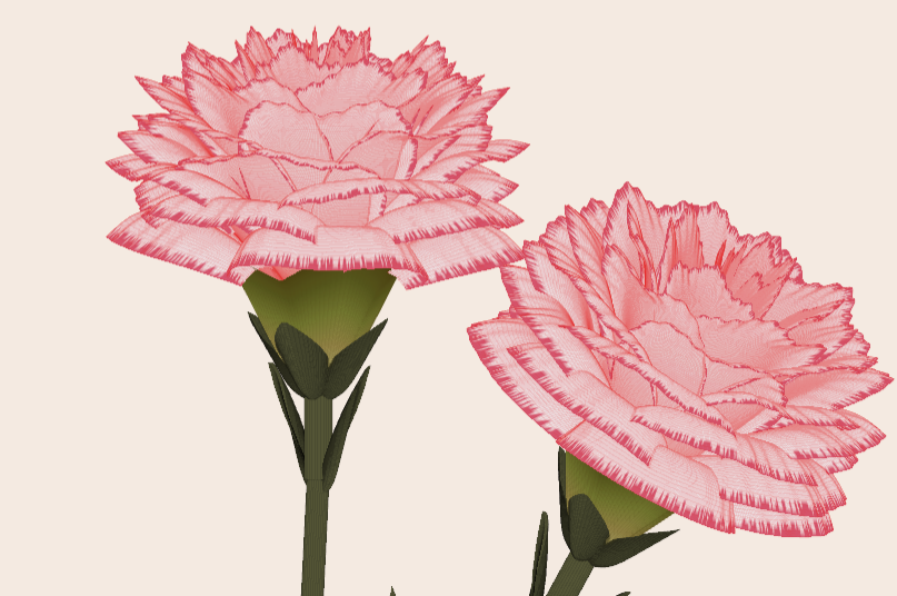
Generate a 3D visualization of carnation flowers
with sepals and stems for celebrating Mother's Day 2026.

function carnation
% CARNATION Generate a 3D visualization of carnation flowers with sepals and stems.
% This code is authored by Zhaoxu Liu / slandarer
% for the purpose of celebrating Mother's Day 2026.
% =========================================================================
% Zhaoxu Liu / slandarer (2026). carnation for Mother's Day
% (https://www.mathworks.com/matlabcentral/fileexchange/183838-carnation-for-mother-s-day),
% MATLAB Central File Exchange. Retrieved May 9, 2026.
% Create figure and axes / 创建图窗及坐标区域
fig = figure('Units','normalized', 'Position',[.3,.1,.4,.8],'Color',[244,234,225]./255);
axes('Parent',fig, 'NextPlot','add', 'DataAspectRatio',[1,1,1],...
'View',[-64, 5.5], 'Position',[0,-.15,1,1], 'Color',[244,234,225]./255, ...
'XColor','none', 'YColor','none', 'ZColor','none');
annotation("textbox", [.05, .8, .9, .2], "String", {"Happy"; "Mother's Day"}, ...
'FontName','Segoe Script', 'FontSize',52, 'FontWeight','bold', 'EdgeColor','none', ...
'HorizontalAlignment','center', 'VerticalAlignment','middle', 'Color',[97,40,20]./255);
xx = linspace(0, 1, 100);
tt = linspace(0, 1, 1e4);
[X, P] = meshgrid(xx, tt);
T1 = P*20*pi;
C1 = 1 - (1 - mod(3.6*T1/pi, 2)).^4./2; % Petal profile / 花瓣形状
S1 = (sin(50*T1)/150 + sin(10*T1)/30).*min(1, max(0, (X - .85)/.1)); % Edge serration / 边缘褶皱和锯齿
Y1 = (- (X.*1.2 - .5).^5.*32 - 1)./15.*P; % Petal curvature / 花瓣弧度
% Petal shape and serration modeling + rotating the planar petal to tilt it
% 花瓣形状和锯齿塑造 + 转动平躺的花瓣令其倾斜
R1 = (C1 + S1).*(X.*sin(P) - Y1.*cos(P))./(P + .5);
H1 = (C1 + S1).*(X.*cos(P) + Y1.*sin(P));
% Convert radius to Cartesian coordinates / 将半径映射为X,Y坐标
X1 = R1.*cos(T1);
Y1 = R1.*sin(T1);
% Colormap for carnation petals / 康乃馨配色
CList1 = [208, 62, 23; 221,146,121; 229,201,202; 233,219,222; 237,223,225]./255;
CMat1 = zeros(1e4, 100, 3);
CMat1(:, :, 1) = repmat(interp1(linspace(0, 1, size(CList1, 1)), CList1(:, 1), linspace(0, 1, 100)), [1e4, 1]);
CMat1(:, :, 2) = repmat(interp1(linspace(0, 1, size(CList1, 1)), CList1(:, 2), linspace(0, 1, 100)), [1e4, 1]);
CMat1(:, :, 3) = repmat(interp1(linspace(0, 1, size(CList1, 1)), CList1(:, 3), linspace(0, 1, 100)), [1e4, 1]);
% Darken edges / 边缘的深色
for i = 1:1e4
tNum = randi([98, 100]);
CMat1(i, tNum:end, 1) = 212./255;
CMat1(i, tNum:end, 2) = 87./255;
CMat1(i, tNum:end, 3) = 113./255;
end
% Rotation matrices / 旋转矩阵
Rx = @(rx) [1, 0, 0; 0, cos(rx), -sin(rx); 0, sin(rx), cos(rx)];
Rz = @(yz) [cos(yz), - sin(yz), 0; sin(yz), cos(yz), 0; 0, 0, 1];
Rx1 = Rx(pi/6); Rz1 = Rz(0);
% Render flower / 绘制康乃馨
surface(X1, Y1, H1 + .3, 'CData',CMat1, 'EdgeAlpha',0.1, 'EdgeColor',[224,39,39]./255, 'FaceColor','interp')
[U1, V1, W1] = matRotate(X1, Y1, H1 + .3, Rx1);
surface(U1 + .7, V1 - .7, W1 - .6, 'CData',CMat1, 'EdgeAlpha',0.1, 'EdgeColor',[224,39,39]./255, 'FaceColor','interp')
% Following the same method as before,
% the profile is designed with four serrated cycles to simulate the four sepals.
% 还是之前的方法,不过让轮廓有4个锯齿状周期来模拟四片花萼
% Sepals generation with 4-lobed pattern / 生成四片花萼(带4个锯齿状周期)
[X, T] = meshgrid(linspace(0, 1, 100), linspace(0, 1, 100).*2*pi);
P2 = T.*0 + pi/8;
C2 = .5 + (.5 - abs(mod(T, pi/2)/pi*2 - .5))*.4;
Y2 = (- (X.*1 - .5).^7.*128 - 1)./15 - .1;
R2 = C2.*(X.*sin(P2) - Y2.*cos(P2));
H2 = C2.*(X.*cos(P2) + Y2.*sin(P2));
X2 = R2.*cos(T);
Y2 = R2.*sin(T);
% Rotate by 90 degrees around the z-axis
% and reduce the size to render the four smaller sepals.
% 绕z轴旋转90度且减小其大小,绘制四片小花萼
% Smaller sepal layer / 绘制四片小花萼(第二层)
P3 = T.*0 + pi/10;
C3 = .3 + (.5 - abs(mod(T + pi/4, pi/2)/pi*2 - .5))*.7;
Y3 = (- (X.*.7 - .5).^7.*128 - 1)./15 - .1;
R3 = C3.*(X.*sin(P3) - Y3.*cos(P3));
H3 = C3.*(X.*cos(P3) + Y3.*sin(P3));
X3 = R3.*cos(T);
Y3 = R3.*sin(T);
% Colormap for sepals / 花托配色
CList2 = [178,173,113; 151,135, 73; 117,123, 50; 86, 89, 29; 75, 65, 17]./255;
CMat2 = zeros(100, 100, 3);
CMat2(:, :, 1) = repmat(interp1(linspace(0, 1, size(CList2, 1)), CList2(:, 1), linspace(0, 1, 100)), [100, 1]);
CMat2(:, :, 2) = repmat(interp1(linspace(0, 1, size(CList2, 1)), CList2(:, 2), linspace(0, 1, 100)), [100, 1]);
CMat2(:, :, 3) = repmat(interp1(linspace(0, 1, size(CList2, 1)), CList2(:, 3), linspace(0, 1, 100)), [100, 1]);
% Render sepals / 绘制花托
surf(X2, Y2, H2.*.8 + .12, 'CData',CMat2, 'EdgeAlpha',0.1, 'EdgeColor',CList2(end,:), 'FaceColor','interp')
surf(X3.*.93, Y3.*.92, H3.*.5 + .02, 'FaceColor',[ 84, 85, 54]./255, 'EdgeAlpha',0.1, 'EdgeColor','k')
[U2, V2, W2] = matRotate(X2, Y2, H2.*.8 + .12, Rx1);
[U3, V3, W3] = matRotate(X3.*.93, Y3.*.92, H3.*.5 + .02, Rx1);
surf(U2 + .7, V2 - .7, W2 - .6, 'CData',CMat2, 'EdgeAlpha',0.1, 'EdgeColor',CList2(end,:), 'FaceColor','interp')
surf(U3 + .7, V3 - .7, W3 - .6, 'FaceColor',[ 84, 85, 54]./255, 'EdgeAlpha',0.1, 'EdgeColor','k')
% A pulse function with two periods is applied
% to the contour to simulate the leaves.
% 让轮廓有2个周期且是脉冲函数,来模拟叶片
P4 = T.*0 + pi/16;
C4 = - abs(mod(T, pi)/pi - .5) + .11;
C4(C4 < 0) = 0; C4 = C4.*10; C4(51:100, :) = C4(51:100, :).*.7;
Y4 = (- (X.*1.01 - .5).^7.*128 - 1)./15 - .03;
R4 = C4.*(X.*sin(P4) - Y4.*cos(P4));
H4 = C4.*(X.*cos(P4) + Y4.*sin(P4));
X4 = R4.*cos(T);
Y4 = R4.*sin(T);
surf(X4 - .1, Y4 + .05, H4 - 2.2, 'FaceColor',[ 84, 85, 54]./255, 'EdgeAlpha',0.1, 'EdgeColor','k')
[U4, V4, W4] = matRotate(X4 - .1, Y4 - .1, H4 + .1, Rz1);
[U4, V4, W4] = matRotate(U4, V4, W4, Rx1);
surf(U4 + .7, V4 - .7 + 1, W4 - .6 - 1.2, 'FaceColor',[ 84, 85, 54]./255, 'EdgeAlpha',0.1, 'EdgeColor','k')
P5 = T.*0 + pi/8;
C5 = - abs(mod(T + pi/6, pi)/pi - .5) + .11;
C5(C5 < 0) = 0; C5 = C5.*5;
Y5 = (- (X.*1.01 - .5).^7.*128 - 1)./15 - .1;
R5 = C5.*(X.*sin(P5) - Y5.*cos(P5));
H5 = C5.*(X.*cos(P5) + Y5.*sin(P5));
X5 = R5.*cos(T);
Y5 = R5.*sin(T);
surf(X5, Y5, H5 - .3, 'FaceColor',[ 84, 85, 54]./255, 'EdgeAlpha',0.1, 'EdgeColor','k')
[U5, V5, W5] = matRotate(X5, Y5, H5+.1, Rx1);
surf(U5 + .7, V5 - .7 + 1/4, W5 - .6 - 1.7/4, 'FaceColor',[ 84, 85, 54]./255, 'EdgeAlpha',0.1, 'EdgeColor','k')
% Render stems / 绘制花杆
P1_1 = [mean(X3(:).*.93), mean(Y3(:).*.92), mean(H3(:).*.5 + .02)];
P1_2 = [mean(X5(:)), mean(Y5(:)), mean(H5(:) - .3)];
P1_3 = [mean(X4(:) - .1), mean(Y4(:) + .05), mean(H4(:) - 2.2)];
P1_3 = (P1_3 - P1_2).*1.4 + P1_2;
[XX1, YY1, ZZ1] = cylinderXYZ(P1_1, P1_2, .05);
[XX2, YY2, ZZ2] = cylinderXYZ(P1_2, P1_3, .04);
surf(XX1, YY1, ZZ1, 'FaceColor',[ 84, 85, 54]./255, 'EdgeAlpha',0.1, 'EdgeColor','k')
surf(XX2, YY2, ZZ2, 'FaceColor',[ 84, 85, 54]./255, 'EdgeAlpha',0.1, 'EdgeColor','k')
P1_1 = [mean(U3(:) + .7), mean(V3(:) - .7), mean(W3(:) - .6)];
P1_2 = [mean(U5(:) + .7), mean(V5(:) - .7 + 1/4), mean(W5(:) - .6 - 1.7/4)];
P1_3 = [mean(U4(:) + .7), mean(V4(:) - .7 + 1), mean(W4(:) - .6 - 1.2)];
P1_3 = (P1_3 - P1_2).*2.4 + P1_2;
[XX1, YY1, ZZ1] = cylinderXYZ(P1_1, P1_2, .05);
[XX2, YY2, ZZ2] = cylinderXYZ(P1_2, P1_3, .04);
surf(XX1, YY1, ZZ1, 'FaceColor',[ 84, 85, 54]./255, 'EdgeAlpha',0.1, 'EdgeColor','k')
surf(XX2, YY2, ZZ2, 'FaceColor',[ 84, 85, 54]./255, 'EdgeAlpha',0.1, 'EdgeColor','k')
% 在任意两点间构建圆柱
function [XX, YY, ZZ] = cylinderXYZ(P1, P2, r)
% CYLINDERXYZ Create a cylinder connecting two 3D points
% [XX, YY, ZZ] = cylinderXYZ(P1, P2, r) generates a cylinder
% of radius r between points P1 and P2.
v = P2 - P1; l = norm(v);
if l < eps, return; end
[XX, YY, ZZ] = cylinder(r, 30); ZZ = ZZ * l;
ddir = [0, 0, 1]; tdir = v / l;
if dot(ddir, tdir) > 0.9999
R = eye(3);
elseif dot(ddir, tdir) < -0.9999
R = [1, 0, 0; 0, -1, 0; 0, 0, -1];
else
av = cross(ddir, tdir); av = av / norm(av);
R = axisRotate(av, acos(dot(ddir, tdir)));
end
for ii = 1:size(XX, 1)
for jj = 1:size(XX, 2)
p = R * [XX(ii, jj); YY(ii, jj); ZZ(ii, jj)];
XX(ii, jj) = p(1) + P1(1);
YY(ii, jj) = p(2) + P1(2);
ZZ(ii, jj) = p(3) + P1(3);
end
end
end
% 通过矩阵旋转数据
function [U, V, W] = matRotate(X, Y, Z, R)
% MATROTATE Apply 3x3 rotation matrix to a set of 3D points
% [U,V,W] = matRotate(X,Y,Z,R) rotates points (X,Y,Z)
% using rotation matrix R.
U = X; V = Y; W = Z;
for ii = 1:numel(X)
v = [X(ii); Y(ii); Z(ii)];
n = R*v; U(ii) = n(1); V(ii) = n(2); W(ii) = n(3);
end
end
% 根据轴-角参数生成旋转矩阵
function R = axisRotate(axis, angle)
% AXISROTATE Compute rotation matrix from axis-angle representation
% R = axisRotate(axis, angle) returns a 3x3 rotation matrix
% for rotating by angle (radians) around the given axis vector.
% Implementation based on Rodrigues' rotation formula.
u = axis(1); v = axis(2); w = axis(3);
c = cos(angle); s = sin(angle);
R = [u^2 + (1-u^2)*c, u*v*(1-c) - w*s, u*w*(1-c) + v*s;
u*v*(1-c) + w*s, v^2 + (1-v^2)*c, v*w*(1-c) - u*s;
u*w*(1-c) - v*s, v*w*(1-c) + u*s, w^2 + (1-w^2)*c];
end
end
I coded this app to solve the 20 or so test cases included with the Cody problem 'visually' and step-by-step. For extra fun, it can also be used to play the game... Any comments or suggestions welcome!
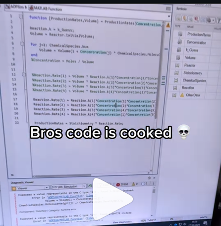
A coworker shared with me a hilarious Instagram post today. A brave bro posted a short video showing his MATLAB code… casually throwing 49,000 errors!
Surprisingly, the video went virial and recieved 250,000+ likes and 800+ comments. You really never know what the Instagram algorithm is thinking, but apparently “my code is absolutely cooked” is a universal developer experience 😂
Last note: Can someone please help this Bro fix his code?
In the sequence of previous suggestion in Meta Cody comment for the 'My Problems' page, I also suggest to add a red alert for new comments in 'My Groups' page.
Thank you in advance.
I can't believe someone put time into this ;-)

I believe that it is very useful and important to know when we have new comments of our own problems. Although I had chosen to receive notifications about my own problems, I only receive them when I am mentioned by @.
Is it possible to add a 'New comment' alert in front of each problem on the 'My Problems' page?

The formula comes from @yuruyurau. (https://x.com/yuruyurau)
digital life 1

figure('Position',[300,50,900,900], 'Color','k');
axes(gcf, 'NextPlot','add', 'Position',[0,0,1,1], 'Color','k');
axis([0, 400, 0, 400])
SHdl = scatter([], [], 2, 'filled','o','w', 'MarkerEdgeColor','none', 'MarkerFaceAlpha',.4);
t = 0;
i = 0:2e4;
x = mod(i, 100);
y = floor(i./100);
k = x./4 - 12.5;
e = y./9 + 5;
o = vecnorm([k; e])./9;
while true
t = t + pi/90;
q = x + 99 + tan(1./k) + o.*k.*(cos(e.*9)./4 + cos(y./2)).*sin(o.*4 - t);
c = o.*e./30 - t./8;
SHdl.XData = (q.*0.7.*sin(c)) + 9.*cos(y./19 + t) + 200;
SHdl.YData = 200 + (q./2.*cos(c));
drawnow
end
digital life 2

figure('Position',[300,50,900,900], 'Color','k');
axes(gcf, 'NextPlot','add', 'Position',[0,0,1,1], 'Color','k');
axis([0, 400, 0, 400])
SHdl = scatter([], [], 2, 'filled','o','w', 'MarkerEdgeColor','none', 'MarkerFaceAlpha',.4);
t = 0;
i = 0:1e4;
x = i;
y = i./235;
e = y./8 - 13;
while true
t = t + pi/240;
k = (4 + sin(y.*2 - t).*3).*cos(x./29);
d = vecnorm([k; e]);
q = 3.*sin(k.*2) + 0.3./k + sin(y./25).*k.*(9 + 4.*sin(e.*9 - d.*3 + t.*2));
SHdl.XData = q + 30.*cos(d - t) + 200;
SHdl.YData = 620 - q.*sin(d - t) - d.*39;
drawnow
end
digital life 3

figure('Position',[300,50,900,900], 'Color','k');
axes(gcf, 'NextPlot','add', 'Position',[0,0,1,1], 'Color','k');
axis([0, 400, 0, 400])
SHdl = scatter([], [], 1, 'filled','o','w', 'MarkerEdgeColor','none', 'MarkerFaceAlpha',.4);
t = 0;
i = 0:1e4;
x = mod(i, 200);
y = i./43;
k = 5.*cos(x./14).*cos(y./30);
e = y./8 - 13;
d = (k.^2 + e.^2)./59 + 4;
a = atan2(k, e);
while true
t = t + pi/20;
q = 60 - 3.*sin(a.*e) + k.*(3 + 4./d.*sin(d.^2 - t.*2));
c = d./2 + e./99 - t./18;
SHdl.XData = q.*sin(c) + 200;
SHdl.YData = (q + d.*9).*cos(c) + 200;
drawnow; pause(1e-2)
end
digital life 4

figure('Position',[300,50,900,900], 'Color','k');
axes(gcf, 'NextPlot','add', 'Position',[0,0,1,1], 'Color','k');
axis([0, 400, 0, 400])
SHdl = scatter([], [], 1, 'filled','o','w', 'MarkerEdgeColor','none', 'MarkerFaceAlpha',.4);
t = 0;
i = 0:4e4;
x = mod(i, 200);
y = i./200;
k = x./8 - 12.5;
e = y./8 - 12.5;
o = (k.^2 + e.^2)./169;
d = .5 + 5.*cos(o);
while true
t = t + pi/120;
SHdl.XData = x + d.*k.*sin(d.*2 + o + t) + e.*cos(e + t) + 100;
SHdl.YData = y./4 - o.*135 + d.*6.*cos(d.*3 + o.*9 + t) + 275;
SHdl.CData = ((d.*sin(k).*sin(t.*4 + e)).^2).'.*[1,1,1];
drawnow;
end
digital life 5

figure('Position',[300,50,900,900], 'Color','k');
axes(gcf, 'NextPlot','add', 'Position',[0,0,1,1], 'Color','k');
axis([0, 400, 0, 400])
SHdl = scatter([], [], 1, 'filled','o','w',...
'MarkerEdgeColor','none', 'MarkerFaceAlpha',.4);
t = 0;
i = 0:1e4;
x = mod(i, 200);
y = i./55;
k = 9.*cos(x./8);
e = y./8 - 12.5;
while true
t = t + pi/120;
d = (k.^2 + e.^2)./99 + sin(t)./6 + .5;
q = 99 - e.*sin(atan2(k, e).*7)./d + k.*(3 + cos(d.^2 - t).*2);
c = d./2 + e./69 - t./16;
SHdl.XData = q.*sin(c) + 200;
SHdl.YData = (q + 19.*d).*cos(c) + 200;
drawnow;
end
digital life 6

clc; clear
figure('Position',[300,50,900,900], 'Color','k');
axes(gcf, 'NextPlot','add', 'Position',[0,0,1,1], 'Color','k');
axis([0, 400, 0, 400])
SHdl = scatter([], [], 2, 'filled','o','w', 'MarkerEdgeColor','none', 'MarkerFaceAlpha',.4);
t = 0;
i = 1:1e4;
y = i./790;
k = y; idx = y < 5;
k(idx) = 6 + sin(bitxor(floor(y(idx)), 1)).*6;
k(~idx) = 4 + cos(y(~idx));
while true
t = t + pi/90;
d = sqrt((k.*cos(i + t./4)).^2 + (y/3-13).^2);
q = y.*k.*cos(i + t./4)./5.*(2 + sin(d.*2 + y - t.*4));
c = d./3 - t./2 + mod(i, 2);
SHdl.XData = q + 90.*cos(c) + 200;
SHdl.YData = 400 - (q.*sin(c) + d.*29 - 170);
drawnow; pause(1e-2)
end
digital life 7

clc; clear
figure('Position',[300,50,900,900], 'Color','k');
axes(gcf, 'NextPlot','add', 'Position',[0,0,1,1], 'Color','k');
axis([0, 400, 0, 400])
SHdl = scatter([], [], 2, 'filled','o','w', 'MarkerEdgeColor','none', 'MarkerFaceAlpha',.4);
t = 0;
i = 1:1e4;
y = i./345;
x = y; idx = y < 11;
x(idx) = 6 + sin(bitxor(floor(x(idx)), 8))*6;
x(~idx) = x(~idx)./5 + cos(x(~idx)./2);
e = y./7 - 13;
while true
t = t + pi/120;
k = x.*cos(i - t./4);
d = sqrt(k.^2 + e.^2) + sin(e./4 + t)./2;
q = y.*k./d.*(3 + sin(d.*2 + y./2 - t.*4));
c = d./2 + 1 - t./2;
SHdl.XData = q + 60.*cos(c) + 200;
SHdl.YData = 400 - (q.*sin(c) + d.*29 - 170);
drawnow; pause(5e-3)
end
digital life 8

clc; clear
figure('Position',[300,50,900,900], 'Color','k');
axes(gcf, 'NextPlot','add', 'Position',[0,0,1,1], 'Color','k');
axis([0, 400, 0, 400])
SHdl{6} = [];
for j = 1:6
SHdl{j} = scatter([], [], 2, 'filled','o','w', 'MarkerEdgeColor','none', 'MarkerFaceAlpha',.3);
end
t = 0;
i = 1:2e4;
k = mod(i, 25) - 12;
e = i./800; m = 200;
theta = pi/3;
R = [cos(theta) -sin(theta); sin(theta) cos(theta)];
while true
t = t + pi/240;
d = 7.*cos(sqrt(k.^2 + e.^2)./3 + t./2);
XY = [k.*4 + d.*k.*sin(d + e./9 + t);
e.*2 - d.*9 - d.*9.*cos(d + t)];
for j = 1:6
XY = R*XY;
SHdl{j}.XData = XY(1,:) + m;
SHdl{j}.YData = XY(2,:) + m;
end
drawnow;
end
digital life 9

clc; clear
figure('Position',[300,50,900,900], 'Color','k');
axes(gcf, 'NextPlot','add', 'Position',[0,0,1,1], 'Color','k');
axis([0, 400, 0, 400])
SHdl{14} = [];
for j = 1:14
SHdl{j} = scatter([], [], 2, 'filled','o','w', 'MarkerEdgeColor','none', 'MarkerFaceAlpha',.1);
end
t = 0;
i = 1:2e4;
k = mod(i, 50) - 25;
e = i./1100; m = 200;
theta = pi/7;
R = [cos(theta) -sin(theta); sin(theta) cos(theta)];
while true
t = t + pi/240;
d = 5.*cos(sqrt(k.^2 + e.^2) - t + mod(i, 2));
XY = [k + k.*d./6.*sin(d + e./3 + t);
90 + e.*d - e./d.*2.*cos(d + t)];
for j = 1:14
XY = R*XY;
SHdl{j}.XData = XY(1,:) + m;
SHdl{j}.YData = XY(2,:) + m;
end
drawnow;
end
In https://www.mathworks.com/matlabcentral/answers/38165-how-to-remove-decimal#comment_3345149 @Luisa asks,
@Cody Team, how can I vote or give a like in great comments?
It seems that there are not such options.
Pure Matlab
82%
Simulink
18%
11 votes
If you have solved a Cody problem before, you have likely seen the Scratch Pad text field below the Solution text field. It provides a quick way to get feedback on your solution before submitting it. Since submitting a solution takes you to a new page, any time a wrong solution is submitted, you have to navigate back to the problem page to try it again.
Instead, I use the Scratch Pad to test my solution repeatedly before submitting. That way, I get to a working solution faster without having to potentially go back and forth many times between the problem page and the wrong-solution page.
Here is my approach:
- Write a tentative solution.
- Copy a test case from the test suite into the Scratch Pad.
- Click the Run Function button—this is immediately below the Scratch Pad and above the Output panel and Submit buttons.
- If the solution does not work, modify the solution code, sometimes putting in disp() lines and/or removing semicolons to trace what the code is doing. Repeat until the solution passes.
- If the solution does work, repeat steps 2 through 4.
- Once there are no more test cases to copy and paste, clean up the code, if necessary (delete disp lines, reinstate all semicolons to suppress output). Click the Run Function button once more, just to make sure I did not break the solution while cleaning it up. Then, click the Submit button.
For problems with large test suites, you may find it useful to copy and paste in multiple test cases per iteration.
Hopefully you find this useful.
Jorge Bernal-AlvizJorge Bernal-Alviz shared the following code that requires R2025a or later:
Test()

function Test()
duration = 10;
numFrames = 800;
frameInterval = duration / numFrames;
w = 400;
t = 0;
i_vals = 1:10000;
x_vals = i_vals;
y_vals = i_vals / 235;
r = linspace(0, 1, 300)';
g = linspace(0, 0.1, 300)';
b = linspace(1, 0, 300)';
r = r * 0.8 + 0.1;
g = g * 0.6 + 0.1;
b = b * 0.9 + 0.1;
customColormap = [r, g, b];
figure('Position', [100, 100, w, w], 'Color', [0, 0, 0]);
axis equal;
axis off;
xlim([0, w]);
ylim([0, w]);
hold on;
colormap default;
colormap(customColormap);
plothandle = scatter([], [], 1, 'filled', 'MarkerFaceAlpha', 0.12);
for i = 1:numFrames
t = t + pi/240;
k = (4 + 3 * sin(y_vals * 2 - t)) .* cos(x_vals / 29);
e = y_vals / 8 - 13;
d = sqrt(k.^2 + e.^2);
c = d - t;
q = 3 * sin(2 * k) + 0.3 ./ (k + 1e-10) + ...
sin(y_vals / 25) .* k .* (9 + 4 * sin(9 * e - 3 * d + 2 * t));
points_x = q + 30 * cos(c) + 200;
points_y = q .* sin(c) + 39 * d - 220;
points_y = w - points_y;
CData = (1 + sin(0.1 * (d - t))) / 3;
CData = max(0, min(1, CData));
set(plothandle, 'XData', points_x, 'YData', points_y, 'CData', CData);
brightness = 0.5 + 0.3 * sin(t * 0.2);
set(plothandle, 'MarkerFaceAlpha', brightness);
drawnow;
pause(frameInterval);
end
end
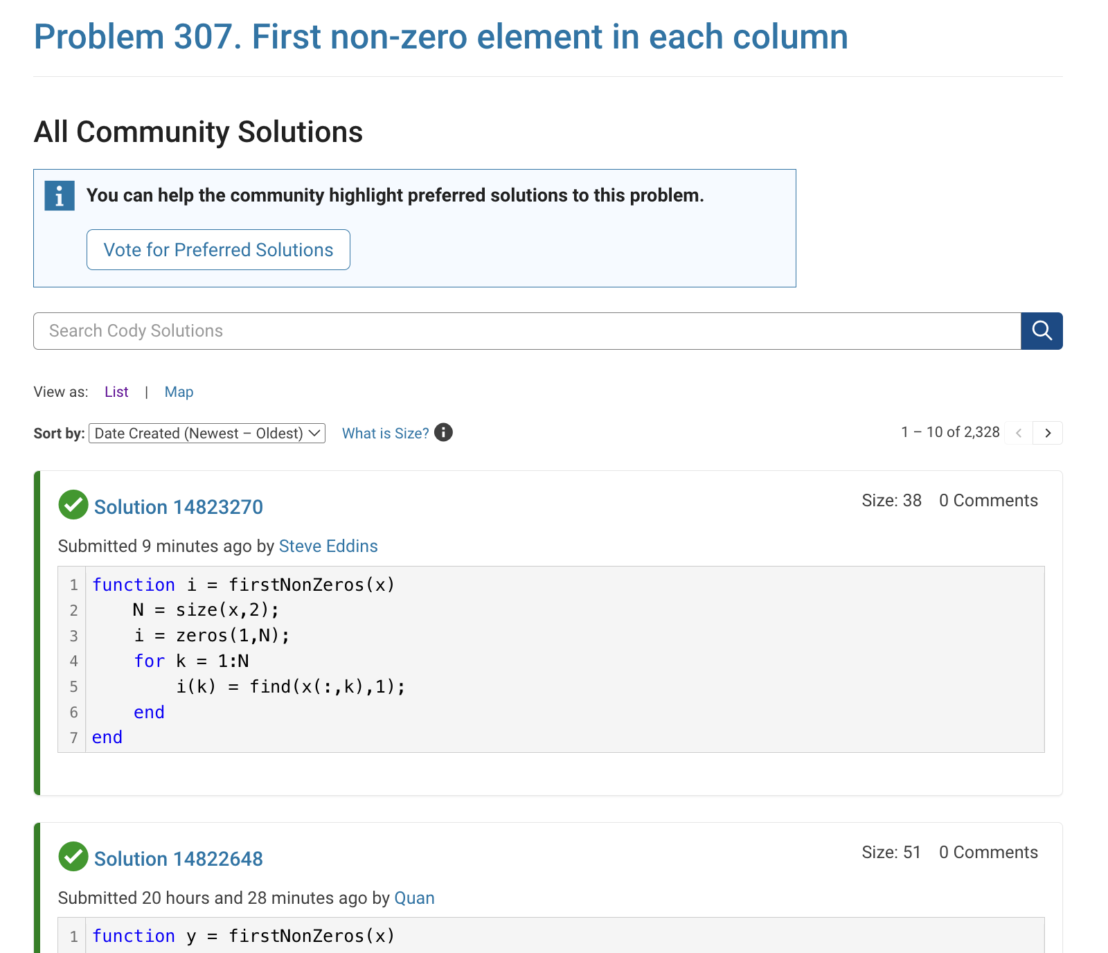
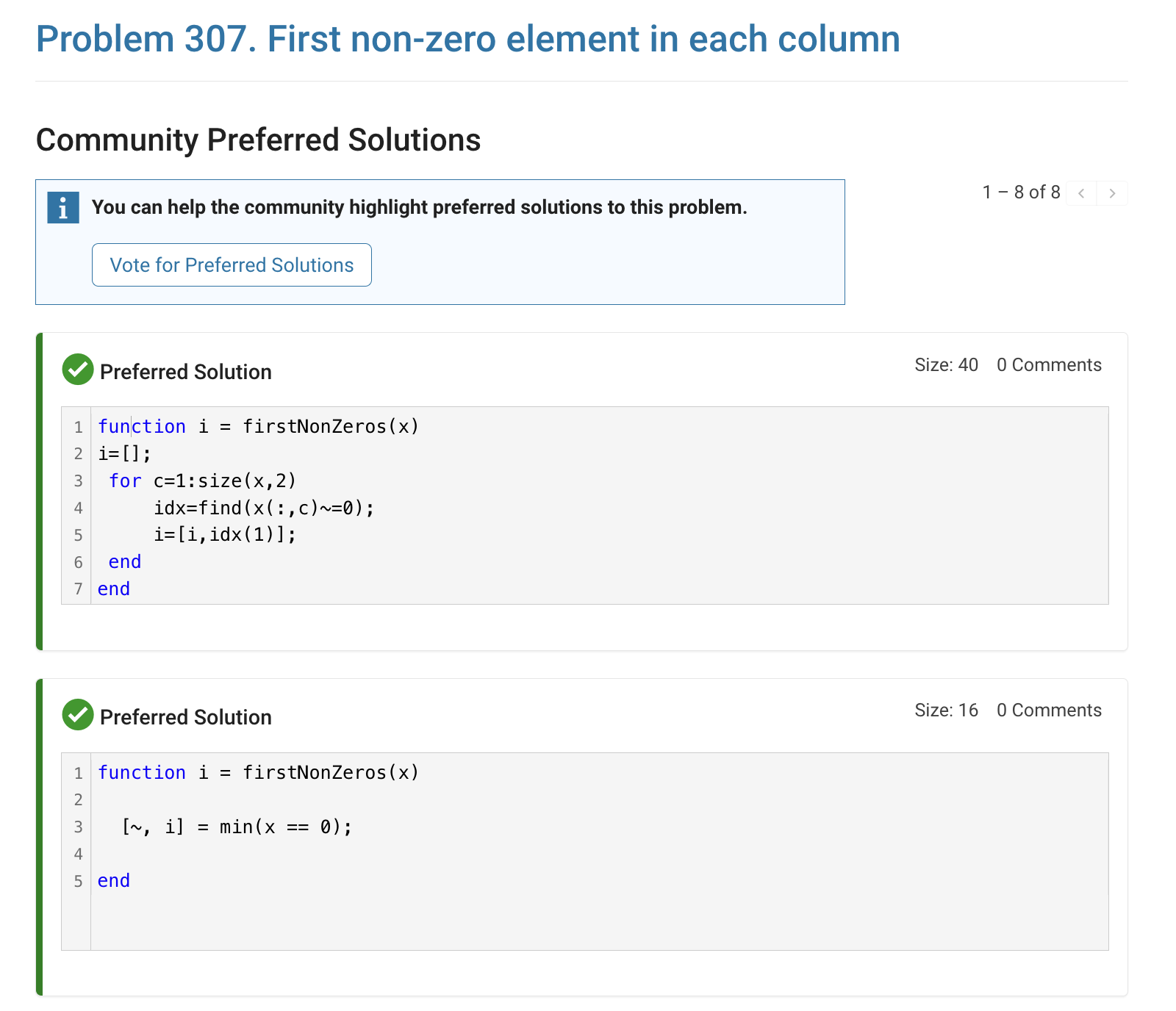
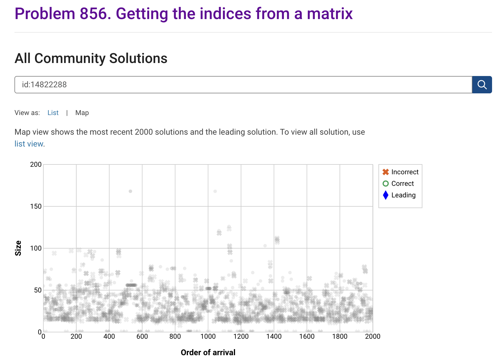
The all-community-solutions view shows the ID of each solution, and you can click on the link to go to the solution.
The preferred-community-solutions view does not show the solution IDs and does not link to the solutions. As far as I can tell, there is no way to get from that view to the solutions. If, for example, you want to go to the solution to leave a comment there, you can't.
All-community-solutions view:
Preferred-community-solutions view, with no solution IDs and no links:
Hi cody fellows,
I already solved more than 500 problems -months ago, last july if I remember well- and get this scholar badge, but then it suddenly disappeared a few weeks later. I then solved a few more problems and it reappeared.
Now I observed it disappeared once more a few days ago.
Have you also noticed this erratic behavior of the scholar badge ? Is it normal and / or intentional ? If not, how to explain it ? (deleted problems ?)
Cheers,
Nicolas
I'm seeing solution maps shown with low-contrast gray colors instead of the correct symbol colors. I have observed this using both Safari and Chrome. Screenshot:
Here is a screenshot of a Cody problem that I just created. The math rendering is poor. (I have since edited the problem to remove the math formatting.)
Are there any code restrictions for programming Cody solutions? I could not find anything mentioned at https://www.mathworks.com/matlabcentral/content/cody/about.html, other than toolbox functions not being available.
Inspired by @xingxingcui's post about old MATLAB versions and @유장's post about an old Easter egg, I thought it might be fun to share some MATLAB-Old-Timer Stories™.
Back in the early 90s, MATLAB had been ported to MacOS, but there were some interesting wrinkles. One that kept me earning my money as a computer lab tutor was that MATLAB required file names to follow Windows standards - no spaces or other special characters. But on a Mac, nothing stopped you from naming your script "hello world - 123.m". The problem came when you tried to run it. MATLAB was essentially doing an eval on the script name, assuming the file name would follow Windows (and MATLAB) naming rules.
So now imagine a lab full of students taking a university course. As is common in many universities, the course was given a numeric code. For whatever historical reason, my school at that time was also using numeric codes for the departments. Despite being told the rules for naming scripts, many students would default to something like "26.165 - 1.1" for problem one on HW1 for the intro applied math course 26.165.
No matter what they did in their script, when they ran it, MATLAB would just say "ans = 25.0650".
Nothing brings you more MATLAB-god credibility as a student tutor than walking over to someone's computer, taking one look at their output, saying "rename your file", and walking away like a boss.
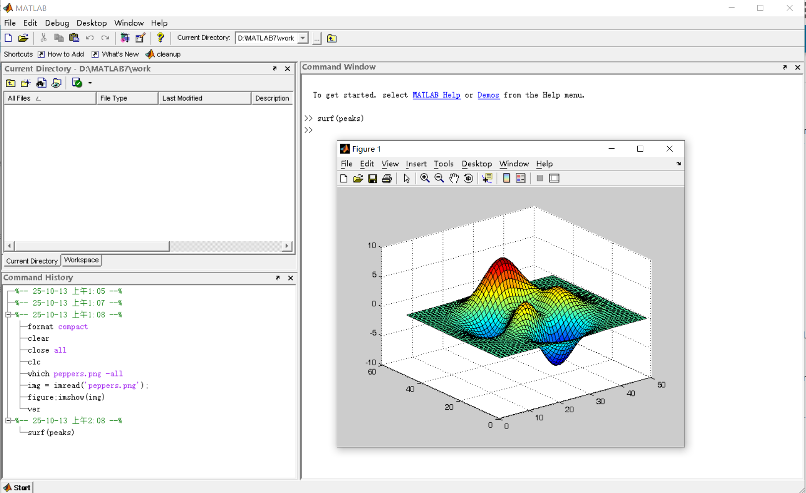
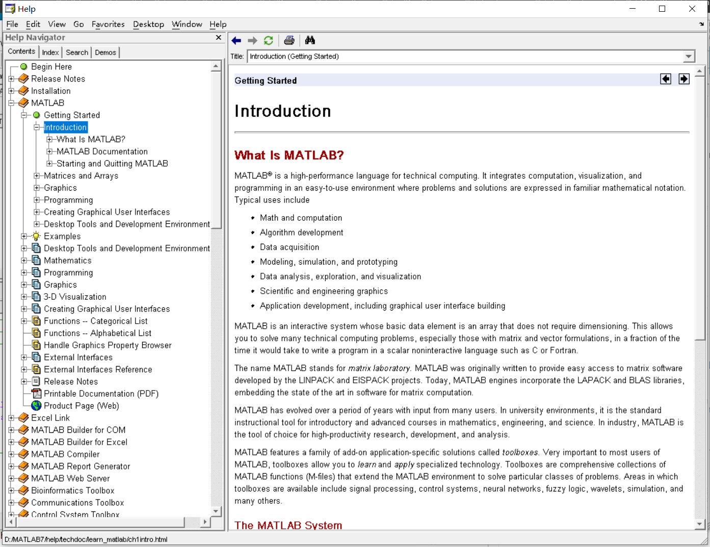
It was 2010 when I was a sophomore in university. I chose to learn MATLAB because of a mathematical modeling competition, and the university provided MATLAB 7.0, a very classic release. To get started, I borrowed many MATLAB books from the library and began by learning simple numerical calculations, plotting, and solving equations. Gradually I was drawn in by MATLAB’s powerful capabilities and became interested; I often used it as a big calculator for fun. That version didn’t have MATLAB Live Script; instead it used MATLAB Notebook (M-Book), which allowed MATLAB functions to be used directly within Microsoft Word, and it also had the Symbolic Math Toolbox’s MuPAD interactive environment. These were later gradually replaced by Live Scripts introduced in R2016a. There are many similar examples...
Out of curiosity, I still have screenshots on my computer showing MATLAB 7.0 running compatibly. I’d love to hear your thoughts?

Do you have a swag signed by Brian Douglas? He does!