Results for
Over the past three weeks, players have been having great fun solving problems, sharing knowledge, and connecting with each other. Did you know over 15,000 solutions have already been submitted?
This is the final week to solve Cody problems and climb the leaderboard in the main round. Remember: solving just one problem in the contest problem group gives you a chance to win MathWorks T-shirts or socks.
🎉 Week 3 Winners:
Weekly Prizes for Contest Problem Group Finishers:
@Umar, @David Hill, @Takumi, @Nicolas, @WANG Zi-Xiang, @Rajvir Singh Gangar, @Roberto, @Boldizsar, @Abi, @Antonio
Weekly Prizes for Contest Problem Group Solvers:
Weekly Prizes for Tips & Tricks Articles:
This week’s prize goes to @Cephas. See the comments from our judge and problem group author @Matt Tearle:
'Some folks have posted deep dives into how to tackle specific problems in the contest set. But others have shared multiple smaller, generally useful tips. This week, I want to congratulate the cumulative contribution of Cool Coder Cephas, who has shared several of my favorite MATLAB techniques, including logical indexing, preallocation, modular arithmetic, and more. Cephas has also given some tips applying these MATLAB techniques to specific contest problems, such as using a convenient MATLAB function to vectorize the Leaderboard problem. Tip for Problem 61059 – Leaderboard for the Nedball World Cup:'
Congratulations to all Week 3 winners! Let’s carry this momentum into the final week!

The formula comes from @yuruyurau. (https://x.com/yuruyurau)
digital life 1

figure('Position',[300,50,900,900], 'Color','k');
axes(gcf, 'NextPlot','add', 'Position',[0,0,1,1], 'Color','k');
axis([0, 400, 0, 400])
SHdl = scatter([], [], 2, 'filled','o','w', 'MarkerEdgeColor','none', 'MarkerFaceAlpha',.4);
t = 0;
i = 0:2e4;
x = mod(i, 100);
y = floor(i./100);
k = x./4 - 12.5;
e = y./9 + 5;
o = vecnorm([k; e])./9;
while true
t = t + pi/90;
q = x + 99 + tan(1./k) + o.*k.*(cos(e.*9)./4 + cos(y./2)).*sin(o.*4 - t);
c = o.*e./30 - t./8;
SHdl.XData = (q.*0.7.*sin(c)) + 9.*cos(y./19 + t) + 200;
SHdl.YData = 200 + (q./2.*cos(c));
drawnow
end
digital life 2

figure('Position',[300,50,900,900], 'Color','k');
axes(gcf, 'NextPlot','add', 'Position',[0,0,1,1], 'Color','k');
axis([0, 400, 0, 400])
SHdl = scatter([], [], 2, 'filled','o','w', 'MarkerEdgeColor','none', 'MarkerFaceAlpha',.4);
t = 0;
i = 0:1e4;
x = i;
y = i./235;
e = y./8 - 13;
while true
t = t + pi/240;
k = (4 + sin(y.*2 - t).*3).*cos(x./29);
d = vecnorm([k; e]);
q = 3.*sin(k.*2) + 0.3./k + sin(y./25).*k.*(9 + 4.*sin(e.*9 - d.*3 + t.*2));
SHdl.XData = q + 30.*cos(d - t) + 200;
SHdl.YData = 620 - q.*sin(d - t) - d.*39;
drawnow
end
digital life 3

figure('Position',[300,50,900,900], 'Color','k');
axes(gcf, 'NextPlot','add', 'Position',[0,0,1,1], 'Color','k');
axis([0, 400, 0, 400])
SHdl = scatter([], [], 1, 'filled','o','w', 'MarkerEdgeColor','none', 'MarkerFaceAlpha',.4);
t = 0;
i = 0:1e4;
x = mod(i, 200);
y = i./43;
k = 5.*cos(x./14).*cos(y./30);
e = y./8 - 13;
d = (k.^2 + e.^2)./59 + 4;
a = atan2(k, e);
while true
t = t + pi/20;
q = 60 - 3.*sin(a.*e) + k.*(3 + 4./d.*sin(d.^2 - t.*2));
c = d./2 + e./99 - t./18;
SHdl.XData = q.*sin(c) + 200;
SHdl.YData = (q + d.*9).*cos(c) + 200;
drawnow; pause(1e-2)
end
digital life 4

figure('Position',[300,50,900,900], 'Color','k');
axes(gcf, 'NextPlot','add', 'Position',[0,0,1,1], 'Color','k');
axis([0, 400, 0, 400])
SHdl = scatter([], [], 1, 'filled','o','w', 'MarkerEdgeColor','none', 'MarkerFaceAlpha',.4);
t = 0;
i = 0:4e4;
x = mod(i, 200);
y = i./200;
k = x./8 - 12.5;
e = y./8 - 12.5;
o = (k.^2 + e.^2)./169;
d = .5 + 5.*cos(o);
while true
t = t + pi/120;
SHdl.XData = x + d.*k.*sin(d.*2 + o + t) + e.*cos(e + t) + 100;
SHdl.YData = y./4 - o.*135 + d.*6.*cos(d.*3 + o.*9 + t) + 275;
SHdl.CData = ((d.*sin(k).*sin(t.*4 + e)).^2).'.*[1,1,1];
drawnow;
end
digital life 5

figure('Position',[300,50,900,900], 'Color','k');
axes(gcf, 'NextPlot','add', 'Position',[0,0,1,1], 'Color','k');
axis([0, 400, 0, 400])
SHdl = scatter([], [], 1, 'filled','o','w',...
'MarkerEdgeColor','none', 'MarkerFaceAlpha',.4);
t = 0;
i = 0:1e4;
x = mod(i, 200);
y = i./55;
k = 9.*cos(x./8);
e = y./8 - 12.5;
while true
t = t + pi/120;
d = (k.^2 + e.^2)./99 + sin(t)./6 + .5;
q = 99 - e.*sin(atan2(k, e).*7)./d + k.*(3 + cos(d.^2 - t).*2);
c = d./2 + e./69 - t./16;
SHdl.XData = q.*sin(c) + 200;
SHdl.YData = (q + 19.*d).*cos(c) + 200;
drawnow;
end
digital life 6

clc; clear
figure('Position',[300,50,900,900], 'Color','k');
axes(gcf, 'NextPlot','add', 'Position',[0,0,1,1], 'Color','k');
axis([0, 400, 0, 400])
SHdl = scatter([], [], 2, 'filled','o','w', 'MarkerEdgeColor','none', 'MarkerFaceAlpha',.4);
t = 0;
i = 1:1e4;
y = i./790;
k = y; idx = y < 5;
k(idx) = 6 + sin(bitxor(floor(y(idx)), 1)).*6;
k(~idx) = 4 + cos(y(~idx));
while true
t = t + pi/90;
d = sqrt((k.*cos(i + t./4)).^2 + (y/3-13).^2);
q = y.*k.*cos(i + t./4)./5.*(2 + sin(d.*2 + y - t.*4));
c = d./3 - t./2 + mod(i, 2);
SHdl.XData = q + 90.*cos(c) + 200;
SHdl.YData = 400 - (q.*sin(c) + d.*29 - 170);
drawnow; pause(1e-2)
end
digital life 7

clc; clear
figure('Position',[300,50,900,900], 'Color','k');
axes(gcf, 'NextPlot','add', 'Position',[0,0,1,1], 'Color','k');
axis([0, 400, 0, 400])
SHdl = scatter([], [], 2, 'filled','o','w', 'MarkerEdgeColor','none', 'MarkerFaceAlpha',.4);
t = 0;
i = 1:1e4;
y = i./345;
x = y; idx = y < 11;
x(idx) = 6 + sin(bitxor(floor(x(idx)), 8))*6;
x(~idx) = x(~idx)./5 + cos(x(~idx)./2);
e = y./7 - 13;
while true
t = t + pi/120;
k = x.*cos(i - t./4);
d = sqrt(k.^2 + e.^2) + sin(e./4 + t)./2;
q = y.*k./d.*(3 + sin(d.*2 + y./2 - t.*4));
c = d./2 + 1 - t./2;
SHdl.XData = q + 60.*cos(c) + 200;
SHdl.YData = 400 - (q.*sin(c) + d.*29 - 170);
drawnow; pause(5e-3)
end
digital life 8

clc; clear
figure('Position',[300,50,900,900], 'Color','k');
axes(gcf, 'NextPlot','add', 'Position',[0,0,1,1], 'Color','k');
axis([0, 400, 0, 400])
SHdl{6} = [];
for j = 1:6
SHdl{j} = scatter([], [], 2, 'filled','o','w', 'MarkerEdgeColor','none', 'MarkerFaceAlpha',.3);
end
t = 0;
i = 1:2e4;
k = mod(i, 25) - 12;
e = i./800; m = 200;
theta = pi/3;
R = [cos(theta) -sin(theta); sin(theta) cos(theta)];
while true
t = t + pi/240;
d = 7.*cos(sqrt(k.^2 + e.^2)./3 + t./2);
XY = [k.*4 + d.*k.*sin(d + e./9 + t);
e.*2 - d.*9 - d.*9.*cos(d + t)];
for j = 1:6
XY = R*XY;
SHdl{j}.XData = XY(1,:) + m;
SHdl{j}.YData = XY(2,:) + m;
end
drawnow;
end
digital life 9

clc; clear
figure('Position',[300,50,900,900], 'Color','k');
axes(gcf, 'NextPlot','add', 'Position',[0,0,1,1], 'Color','k');
axis([0, 400, 0, 400])
SHdl{14} = [];
for j = 1:14
SHdl{j} = scatter([], [], 2, 'filled','o','w', 'MarkerEdgeColor','none', 'MarkerFaceAlpha',.1);
end
t = 0;
i = 1:2e4;
k = mod(i, 50) - 25;
e = i./1100; m = 200;
theta = pi/7;
R = [cos(theta) -sin(theta); sin(theta) cos(theta)];
while true
t = t + pi/240;
d = 5.*cos(sqrt(k.^2 + e.^2) - t + mod(i, 2));
XY = [k + k.*d./6.*sin(d + e./3 + t);
90 + e.*d - e./d.*2.*cos(d + t)];
for j = 1:14
XY = R*XY;
SHdl{j}.XData = XY(1,:) + m;
SHdl{j}.YData = XY(2,:) + m;
end
drawnow;
end
In just two weeks, the competition has become both intense and friendly as participants race to climb the team leaderboard, especially in Team Creative, where @Mehdi Dehghan currently leads with 1400+ points, followed by @Vasilis Bellos with 900+ points.
There’s still plenty of time to participate before the contest's main round ends on December 7. Solving just one problem in the contest problem group gives you a chance to win MathWorks T-shirts or socks. Completing the entire problem group not only boosts your odds but also helps your team win.
🎉 Week 2 Winners:
Weekly Prizes for Contest Problem Group Finishers:
@Cephas, @Athi, @Bin Jiang, @Armando Longobardi, @Simone, @Maxi, @Pietro, @Hong Son, @Salvatore, @KARUPPASAMYPANDIYAN M
Weekly Prizes for Contest Problem Group Solvers:
Weekly Prizes for Tips & Tricks Articles:
This week’s prize goes to @Athi for the highly detailed post Solving Systematically The Clueless - Lord Ned in the Game Room.
Comment from the judge:
Shortly after the problem set dropped, several folks recognized that the final problem, "Clueless", was a step above the rest in difficulty. So, not surprisingly, there were a few posts in the discussion boards related to how to tackle this problem. Athi, of the Cool Coders, really dug deep into how the rules and strategies could be turned into an algorithm. There's always more than one way to tackle any difficult programming problem, so it was nice to see some discussion in the comments on different ways you can structure the array that represents your knowledge of who has which cards.
Congratulations to all Week 2 winners! Let’s keep the momentum going!

% Recreation of Saturn photo
figure('Color', 'k', 'Position', [100, 100, 800, 800]);
ax = axes('Color', 'k', 'XColor', 'none', 'YColor', 'none', 'ZColor', 'none');
hold on;
% Create the planet sphere
[x, y, z] = sphere(150);
% Saturn colors - pale yellow/cream gradient
saturn_radius = 1;
% Create color data based on latitude for gradient effect
lat = asin(z);
color_data = rescale(lat, 0.3, 0.9);
% Plot Saturn with smooth shading
planet = surf(x*saturn_radius, y*saturn_radius, z*saturn_radius, ...
color_data, ...
'EdgeColor', 'none', ...
'FaceColor', 'interp', ...
'FaceLighting', 'gouraud', ...
'AmbientStrength', 0.3, ...
'DiffuseStrength', 0.6, ...
'SpecularStrength', 0.1);
% Use a cream/pale yellow colormap for Saturn
cream_map = [linspace(0.4, 0.95, 256)', ...
linspace(0.35, 0.9, 256)', ...
linspace(0.2, 0.7, 256)'];
colormap(cream_map);
% Create the ring system
n_points = 300;
theta = linspace(0, 2*pi, n_points);
% Define ring structure (inner radius, outer radius, brightness)
rings = [
1.2, 1.4, 0.7; % Inner ring
1.45, 1.65, 0.8; % A ring
1.7, 1.85, 0.5; % Cassini division (darker)
1.9, 2.3, 0.9; % B ring (brightest)
2.35, 2.5, 0.6; % C ring
2.55, 2.8, 0.4; % Outer rings (fainter)
];
% Create rings as patches
for i = 1:size(rings, 1)
r_inner = rings(i, 1);
r_outer = rings(i, 2);
brightness = rings(i, 3);
% Create ring coordinates
x_inner = r_inner * cos(theta);
y_inner = r_inner * sin(theta);
x_outer = r_outer * cos(theta);
y_outer = r_outer * sin(theta);
% Front side of rings
ring_x = [x_inner, fliplr(x_outer)];
ring_y = [y_inner, fliplr(y_outer)];
ring_z = zeros(size(ring_x));
% Color based on brightness
ring_color = brightness * [0.9, 0.85, 0.7];
fill3(ring_x, ring_y, ring_z, ring_color, ...
'EdgeColor', 'none', ...
'FaceAlpha', 0.7, ...
'FaceLighting', 'gouraud', ...
'AmbientStrength', 0.5);
end
% Add some texture/gaps in the rings using scatter
n_particles = 3000;
r_particles = 1.2 + rand(1, n_particles) * 1.6;
theta_particles = rand(1, n_particles) * 2 * pi;
x_particles = r_particles .* cos(theta_particles);
y_particles = r_particles .* sin(theta_particles);
z_particles = (rand(1, n_particles) - 0.5) * 0.02;
% Vary particle brightness
particle_colors = repmat([0.8, 0.75, 0.6], n_particles, 1) .* ...
(0.5 + 0.5*rand(n_particles, 1));
scatter3(x_particles, y_particles, z_particles, 1, particle_colors, ...
'filled', 'MarkerFaceAlpha', 0.3);
% Add dramatic outer halo effect - multiple layers extending far out
n_glow = 20;
for i = 1:n_glow
glow_radius = 1 + i*0.35; % Extend much farther
alpha_val = 0.08 / sqrt(i); % More visible, slower falloff
% Color gradient from cream to blue/purple at outer edges
if i <= 8
glow_color = [0.9, 0.85, 0.7]; % Warm cream/yellow
else
% Gradually shift to cooler colors
mix = (i - 8) / (n_glow - 8);
glow_color = (1-mix)*[0.9, 0.85, 0.7] + mix*[0.6, 0.65, 0.85];
end
surf(x*glow_radius, y*glow_radius, z*glow_radius, ...
ones(size(x)), ...
'EdgeColor', 'none', ...
'FaceColor', glow_color, ...
'FaceAlpha', alpha_val, ...
'FaceLighting', 'none');
end
% Add extensive glow to rings - make it much more dramatic
n_ring_glow = 12;
for i = 1:n_ring_glow
glow_scale = 1 + i*0.15; % Extend farther
alpha_ring = 0.12 / sqrt(i); % More visible
for j = 1:size(rings, 1)
r_inner = rings(j, 1) * glow_scale;
r_outer = rings(j, 2) * glow_scale;
brightness = rings(j, 3) * 0.5 / sqrt(i);
x_inner = r_inner * cos(theta);
y_inner = r_inner * sin(theta);
x_outer = r_outer * cos(theta);
y_outer = r_outer * sin(theta);
ring_x = [x_inner, fliplr(x_outer)];
ring_y = [y_inner, fliplr(y_outer)];
ring_z = zeros(size(ring_x));
% Color gradient for ring glow
if i <= 6
ring_color = brightness * [0.9, 0.85, 0.7];
else
mix = (i - 6) / (n_ring_glow - 6);
ring_color = brightness * ((1-mix)*[0.9, 0.85, 0.7] + mix*[0.65, 0.7, 0.9]);
end
fill3(ring_x, ring_y, ring_z, ring_color, ...
'EdgeColor', 'none', ...
'FaceAlpha', alpha_ring, ...
'FaceLighting', 'none');
end
end
% Add diffuse glow particles for atmospheric effect
n_glow_particles = 8000;
glow_radius_particles = 1.5 + rand(1, n_glow_particles) * 5;
theta_glow = rand(1, n_glow_particles) * 2 * pi;
phi_glow = acos(2*rand(1, n_glow_particles) - 1);
x_glow = glow_radius_particles .* sin(phi_glow) .* cos(theta_glow);
y_glow = glow_radius_particles .* sin(phi_glow) .* sin(theta_glow);
z_glow = glow_radius_particles .* cos(phi_glow);
% Color particles based on distance - cooler colors farther out
particle_glow_colors = zeros(n_glow_particles, 3);
for i = 1:n_glow_particles
dist = glow_radius_particles(i);
if dist < 3
particle_glow_colors(i,:) = [0.9, 0.85, 0.7];
else
mix = (dist - 3) / 4;
particle_glow_colors(i,:) = (1-mix)*[0.9, 0.85, 0.7] + mix*[0.5, 0.6, 0.9];
end
end
scatter3(x_glow, y_glow, z_glow, rand(1, n_glow_particles)*2+0.5, ...
particle_glow_colors, 'filled', 'MarkerFaceAlpha', 0.05);
% Lighting setup
light('Position', [-3, -2, 4], 'Style', 'infinite', ...
'Color', [1, 1, 0.95]);
light('Position', [2, 3, 2], 'Style', 'infinite', ...
'Color', [0.3, 0.3, 0.4]);
% Camera and view settings
axis equal off;
view([-35, 25]); % Angle to match saturn_photo.jpg - more dramatic tilt
camva(10); % Field of view - slightly wider to show full halo
xlim([-8, 8]); % Expanded to show outer halo
ylim([-8, 8]);
zlim([-8, 8]);
% Material properties
material dull;
title('Saturn - Left click: Rotate | Right click: Pan | Scroll: Zoom', 'Color', 'w', 'FontSize', 12);
% Enable interactive camera controls
cameratoolbar('Show');
cameratoolbar('SetMode', 'orbit'); % Start in rotation mode

% Custom mouse controls
set(gcf, 'WindowButtonDownFcn', @mouseDown);
function mouseDown(src, ~)
selType = get(src, 'SelectionType');
switch selType
case 'normal' % Left click - rotate
cameratoolbar('SetMode', 'orbit');
rotate3d on;
case 'alt' % Right click - pan
cameratoolbar('SetMode', 'pan');
pan on;
end
end
Hello,
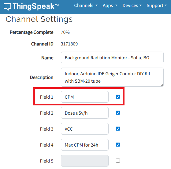
I have Arduino DIY Geiger Counter, that uploads data to my channel here in ThingSpeak (3171809), using ESP8266 WiFi board. It sends CPM values (counts per minute), Dose, VCC and Max CPM for 24h. They are assignet to Field from 1 to 4 respectively. How can I duplicate Field 1, so I could create different time chart for the same measured unit? Or should I duplicate Field 1 chart, and how? I tried to find the answer here in the blog, but I couldn't.
I have to say that I'm not an engineer or coder, just can simply load some Arduino sketches and few more things, so I'll be very thankfull if someone could explain like for non-IT users.
Regards,
Emo
In just one week, we have hit an amazing milestone: 500+ players registered and 5000+ solutions submitted! We’ve also seen fantastic Tips & Tricks articles rolling in, making this contest a true community learning experience.
And here’s the best part: you don’t need to be a top-ranked player to win. To encourage more casual and first-time players to jump in, we’re introducing new weekly prizes starting Week 2!
New Casual Player Prizes:
- 5 extra MathWorks T-shirts or socks will be awarded every week.
- All you need to qualify is to register and solve one problem in the Contest Problem Group.
Jump in, try a few problems, and don’t be shy to ask questions in your team’s channel. You might walk away with a prize!
Week 1 Winners:
Weekly Prizes for Contest Problem Group Finishers:
@Mazhar, @Julien, @Mohammad Aryayi, @Pawel, @Mehdi Dehghan, @Christian Schröder, @Yolanda, @Dev Gupta, @Tomoaki Takagi, @Stefan Abendroth
Weekly Prizes for Tips & Tricks Articles:
We had a lot of people share useful tips (including some personal favorite MATLAB tricks). But Vasilis Bellos went *deep* into the Bridges of Nedsburg problem. Fittingly for a Creative Coder, his post was innovative and entertaining, while also cleverly sneaking in some hints on a neat solution method that wasn't advertised in the problem description.
Congratulations to all Week 1 winners! Prizes will be awarded after the contest ends. Let’s keep the momentum going!
Experimenting with Agentic AI
44%
I am an AI skeptic
0%
AI is banned at work
11%
I am happy with Conversational AI
44%
9 votes

It’s exciting to dive into a new dataset full of unfamiliar variables but it can also be overwhelming if you’re not sure where to start. Recently, I discovered some new interactive features in MATLAB live scripts that make it much easier to get an overview of your data. With just a few clicks, you can display sparklines and summary statistics using table variables, sort and filter variables, and even have MATLAB generate the corresponding code for reproducibility.
The Graphics and App Building blog published an article that walks through these features showing how to explore, clean, and analyze data—all without writing any code.
If you’re interested in streamlining your exploratory data analysis or want to see what’s new in live scripts, you might find it helpful:
If you’ve tried these features or have your own tips for quick data exploration in MATLAB, I’d love to hear your thoughts!
Pure Matlab
82%
Simulink
18%
11 votes
What a fantastic start to Cody Contest 2025! In just 2 days, over 300 players joined the fun, and we already have our first contest group finishers. A big shoutout to the first finisher from each team:
- Team Creative Coders: @Mehdi Dehghan
- Team Cool Coders: @Pawel
- Team Relentless Coders: @David Hill
- 🏆 First finisher overall: Mehdi Dehghan
Other group finishers: @Bin Jiang (Relentless), @Mazhar (Creative), @Vasilis Bellos (Creative), @Stefan Abendroth (Creative), @Armando Longobardi (Cool), @Cephas (Cool)
Kudos to all group finishers! 🎉
Reminder to finishers: The goal of Cody Contest is learning together. Share hints (not full solutions) to help your teammates complete the problem group. The winning team will be the one with the most group finishers — teamwork matters!
To all players: Don’t be shy about asking for help! When you do, show your work — include your code, error messages, and any details needed for others to reproduce your results.
Keep solving, keep sharing, and most importantly — have fun!
The main round of Cody Contest 2025 kicks off today! Whether you’re a beginner or a seasoned solver, now’s your time to shine.
Here’s how to join the fun:
- Pick your team — choose one that matches your coding personality.
- Solve Cody problems — gain points and climb the leaderboard.
- Finish the Contest Problem Group — help your team win and unlock chances for weekly prizes by finishing the Cody Contest 2025 problem group.
- Share Tips & Tricks — post your insights to win a coveted MathWorks Yeti Bottle.
- Bonus Round — 2 players from each team will be invited to a fun live code-along event!
- Watch Party – join the big watch event to see how top players tackle Cody problems
Contest Timeline:
- Main Round: Nov 10 – Dec 7, 2025
- Bonus Round: Dec 8 – Dec 19, 2025
Big prizes await — MathWorks swag, Amazon gift cards, and shiny virtual badges!
We look forward to seeing you in the contest — learn, compete, and have fun!
Jorge Bernal-AlvizJorge Bernal-Alviz shared the following code that requires R2025a or later:
Test()

function Test()
duration = 10;
numFrames = 800;
frameInterval = duration / numFrames;
w = 400;
t = 0;
i_vals = 1:10000;
x_vals = i_vals;
y_vals = i_vals / 235;
r = linspace(0, 1, 300)';
g = linspace(0, 0.1, 300)';
b = linspace(1, 0, 300)';
r = r * 0.8 + 0.1;
g = g * 0.6 + 0.1;
b = b * 0.9 + 0.1;
customColormap = [r, g, b];
figure('Position', [100, 100, w, w], 'Color', [0, 0, 0]);
axis equal;
axis off;
xlim([0, w]);
ylim([0, w]);
hold on;
colormap default;
colormap(customColormap);
plothandle = scatter([], [], 1, 'filled', 'MarkerFaceAlpha', 0.12);
for i = 1:numFrames
t = t + pi/240;
k = (4 + 3 * sin(y_vals * 2 - t)) .* cos(x_vals / 29);
e = y_vals / 8 - 13;
d = sqrt(k.^2 + e.^2);
c = d - t;
q = 3 * sin(2 * k) + 0.3 ./ (k + 1e-10) + ...
sin(y_vals / 25) .* k .* (9 + 4 * sin(9 * e - 3 * d + 2 * t));
points_x = q + 30 * cos(c) + 200;
points_y = q .* sin(c) + 39 * d - 220;
points_y = w - points_y;
CData = (1 + sin(0.1 * (d - t))) / 3;
CData = max(0, min(1, CData));
set(plothandle, 'XData', points_x, 'YData', points_y, 'CData', CData);
brightness = 0.5 + 0.3 * sin(t * 0.2);
set(plothandle, 'MarkerFaceAlpha', brightness);
drawnow;
pause(frameInterval);
end
end
From my experience, MATLAB's Deep Learning Toolbox is quite user-friendly, but it still falls short of libraries like PyTorch in many respects. Most users tend to choose PyTorch because of its flexibility, efficiency, and rich support for many mathematical operators. In recent years, the number of dlarray-compatible mathematical functions added to the toolbox has been very limited, which makes it difficult to experiment with many custom networks. For example, svd is currently not supported for dlarray inputs.
This link (List of Functions with dlarray Support - MATLAB & Simulink) lists all functions that support dlarray as of R2026a — only around 200 functions (including toolbox-specific ones). I would like to see support for many more fundamental mathematical functions so that users have greater freedom when building and researching custom models. For context, the core MATLAB mathematics module contains roughly 600 functions, and many application domains build on that foundation.
I hope MathWorks will prioritize and accelerate expanding dlarray support for basic math functions. Doing so would significantly increase the Deep Learning Toolbox's utility and appeal for researchers and practitioners.
Thank you.
Run MATLAB using AI applications by leveraging MCP. This MCP server for MATLAB supports a wide range of coding agents like Claude Code and Visual Studio Code.
Check it out and share your experiences below. Have fun!
GitHub repo: https://github.com/matlab/matlab-mcp-core-server
Yann Debray's blog post: https://blogs.mathworks.com/deep-learning/2025/11/03/releasing-the-matlab-mcp-core-server-on-github/
Pick a team, solve Cody problems, and share your best tips and tricks. Whether you’re a beginner or a seasoned MATLAB user, you’ll have fun learning, connecting with others, and competing for amazing prizes, including MathWorks swags, Amazon gift cards, and virtual badges.
How to Participate
- Join a team that matches your coding personality
- Solve Cody problems, complete the contest problem group, or share Tips & Tricks articles
- Bonus Round: Two top players from each team will be invited to a fun code-along event
Contest Timeline
- Main Round: Nov 10 – Dec 7, 2025
- Bonus Round: Dec 8 – Dec 19, 2025
Prizes (updated 11/19)
- (New prize) Solving just one problem in the contest problem group gives you a chance to win MathWorks T-shirts or socks each week.
- Finishing the entire problem group will greatly increase your chances—while helping your team win.
- Share high-quality Tips & Tricks articles to earn you a coveted MathWorks Yeti Bottle.
- Become a top finisher in your team to win Amazon gift cards and an invitation to the bonus round.
как я получил api Token
I just learned you can access MATLAB Online from the following shortcut in your web browser: https://matlab.new
Thanks @Yann Debray
From his recent blog post: pip & uv in MATLAB Online » Artificial Intelligence - MATLAB & Simulink
Hey everyone,
I’m currently working with MATLAB R2025b and using the MQTT blocks from the Industrial Communication Toolbox inside Simulink. I’ve run into an issue that’s driving me a bit crazy, and I’m not sure if it’s a bug or if I’m missing something obvious.
Here’s what’s happening:
- I open the MQTT Configure block.
- I fill out all the required fields — Broker address, Port, Client ID, Username, and Password.
- When I click Test Connection, it says “Connection established successfully.” So far so good.
- Then I click Apply, close the dialog, set the topic name, and try to run the simulation.
- At this point, I get the following error:Caused by: Invalid value for 'ClientID', 'Username' or 'Password'.
- When I reopen the MQTT config block, I notice that the Password field is empty again — even though I definitely entered it before and the connection test worked earlier.
It seems like Simulink is somehow not saving the password after hitting Apply, which leads to the authentication error during simulation.
Has anyone else faced this? Is this a bug in R2025b, or do I need to configure something differently to make the password persist?
Would really appreciate any insights, workarounds, or confirmations from anyone who has used MQTT in Simulink recently.
Thanks in advance!
I'm working on training neural networks without backpropagation / automatic differentiation, using locally derived analytic forms of update rules. Given that this allows a direct formula to be derived for the update rule, it removes alot of the overhead that is otherwise required from automatic differentiation.
However, matlab's functionalities for neural networks are currently solely based around backpropagation and automatic differentiation, such as the dlgradient function and requiring everything to be dlarrays during training.
I have two main requests, specifically for functions that perform a single operation within a single layer of a neural network, such as "dlconv", "fullyconnect", "maxpool", "avgpool", "relu", etc:
- these functions should also allow normal gpuArray data instead of requiring everything to be dlarrays.
- these functions are currently designed to only perform the forward pass. I request that these also be designed to perform the backward pass if user requests. There can be another input user flag that can be "forward" (default) or "backward", and then the function should have all the necessary inputs to perform that operation (e.g. for "avgpool" forward pass it only needs the avgpool input data and the avgpool parameters, but for the "avgpool" backward pass it needs the deriviative w.r.t. the avgpool output data, the avgpool parameters, and the original data dimensions). I know that there is a maxunpool function that achieves this for maxpool, but it has significant issues when trying to use it this way instead of by backpropagation in a dlgradient type layer, see (https://www.mathworks.com/matlabcentral/answers/2179587-making-a-custom-way-to-train-cnns-and-i-am-noticing-that-avgpool-is-significantly-faster-than-maxpo?s_tid=srchtitle).
I don't know how many people would benefit from this feature, and someone could always spend their time creating these functionalities themselves by matlab scripts, cuDNN mex, etc., but regardless it would be nice for matlab to have this allowable for more customizable neural net training.
Inspired by @xingxingcui's post about old MATLAB versions and @유장's post about an old Easter egg, I thought it might be fun to share some MATLAB-Old-Timer Stories™.
Back in the early 90s, MATLAB had been ported to MacOS, but there were some interesting wrinkles. One that kept me earning my money as a computer lab tutor was that MATLAB required file names to follow Windows standards - no spaces or other special characters. But on a Mac, nothing stopped you from naming your script "hello world - 123.m". The problem came when you tried to run it. MATLAB was essentially doing an eval on the script name, assuming the file name would follow Windows (and MATLAB) naming rules.
So now imagine a lab full of students taking a university course. As is common in many universities, the course was given a numeric code. For whatever historical reason, my school at that time was also using numeric codes for the departments. Despite being told the rules for naming scripts, many students would default to something like "26.165 - 1.1" for problem one on HW1 for the intro applied math course 26.165.
No matter what they did in their script, when they ran it, MATLAB would just say "ans = 25.0650".
Nothing brings you more MATLAB-god credibility as a student tutor than walking over to someone's computer, taking one look at their output, saying "rename your file", and walking away like a boss.