Results for

The formula comes from @yuruyurau. (https://x.com/yuruyurau)
digital life 1

figure('Position',[300,50,900,900], 'Color','k');
axes(gcf, 'NextPlot','add', 'Position',[0,0,1,1], 'Color','k');
axis([0, 400, 0, 400])
SHdl = scatter([], [], 2, 'filled','o','w', 'MarkerEdgeColor','none', 'MarkerFaceAlpha',.4);
t = 0;
i = 0:2e4;
x = mod(i, 100);
y = floor(i./100);
k = x./4 - 12.5;
e = y./9 + 5;
o = vecnorm([k; e])./9;
while true
t = t + pi/90;
q = x + 99 + tan(1./k) + o.*k.*(cos(e.*9)./4 + cos(y./2)).*sin(o.*4 - t);
c = o.*e./30 - t./8;
SHdl.XData = (q.*0.7.*sin(c)) + 9.*cos(y./19 + t) + 200;
SHdl.YData = 200 + (q./2.*cos(c));
drawnow
end
digital life 2

figure('Position',[300,50,900,900], 'Color','k');
axes(gcf, 'NextPlot','add', 'Position',[0,0,1,1], 'Color','k');
axis([0, 400, 0, 400])
SHdl = scatter([], [], 2, 'filled','o','w', 'MarkerEdgeColor','none', 'MarkerFaceAlpha',.4);
t = 0;
i = 0:1e4;
x = i;
y = i./235;
e = y./8 - 13;
while true
t = t + pi/240;
k = (4 + sin(y.*2 - t).*3).*cos(x./29);
d = vecnorm([k; e]);
q = 3.*sin(k.*2) + 0.3./k + sin(y./25).*k.*(9 + 4.*sin(e.*9 - d.*3 + t.*2));
SHdl.XData = q + 30.*cos(d - t) + 200;
SHdl.YData = 620 - q.*sin(d - t) - d.*39;
drawnow
end
digital life 3

figure('Position',[300,50,900,900], 'Color','k');
axes(gcf, 'NextPlot','add', 'Position',[0,0,1,1], 'Color','k');
axis([0, 400, 0, 400])
SHdl = scatter([], [], 1, 'filled','o','w', 'MarkerEdgeColor','none', 'MarkerFaceAlpha',.4);
t = 0;
i = 0:1e4;
x = mod(i, 200);
y = i./43;
k = 5.*cos(x./14).*cos(y./30);
e = y./8 - 13;
d = (k.^2 + e.^2)./59 + 4;
a = atan2(k, e);
while true
t = t + pi/20;
q = 60 - 3.*sin(a.*e) + k.*(3 + 4./d.*sin(d.^2 - t.*2));
c = d./2 + e./99 - t./18;
SHdl.XData = q.*sin(c) + 200;
SHdl.YData = (q + d.*9).*cos(c) + 200;
drawnow; pause(1e-2)
end
digital life 4

figure('Position',[300,50,900,900], 'Color','k');
axes(gcf, 'NextPlot','add', 'Position',[0,0,1,1], 'Color','k');
axis([0, 400, 0, 400])
SHdl = scatter([], [], 1, 'filled','o','w', 'MarkerEdgeColor','none', 'MarkerFaceAlpha',.4);
t = 0;
i = 0:4e4;
x = mod(i, 200);
y = i./200;
k = x./8 - 12.5;
e = y./8 - 12.5;
o = (k.^2 + e.^2)./169;
d = .5 + 5.*cos(o);
while true
t = t + pi/120;
SHdl.XData = x + d.*k.*sin(d.*2 + o + t) + e.*cos(e + t) + 100;
SHdl.YData = y./4 - o.*135 + d.*6.*cos(d.*3 + o.*9 + t) + 275;
SHdl.CData = ((d.*sin(k).*sin(t.*4 + e)).^2).'.*[1,1,1];
drawnow;
end
digital life 5

figure('Position',[300,50,900,900], 'Color','k');
axes(gcf, 'NextPlot','add', 'Position',[0,0,1,1], 'Color','k');
axis([0, 400, 0, 400])
SHdl = scatter([], [], 1, 'filled','o','w',...
'MarkerEdgeColor','none', 'MarkerFaceAlpha',.4);
t = 0;
i = 0:1e4;
x = mod(i, 200);
y = i./55;
k = 9.*cos(x./8);
e = y./8 - 12.5;
while true
t = t + pi/120;
d = (k.^2 + e.^2)./99 + sin(t)./6 + .5;
q = 99 - e.*sin(atan2(k, e).*7)./d + k.*(3 + cos(d.^2 - t).*2);
c = d./2 + e./69 - t./16;
SHdl.XData = q.*sin(c) + 200;
SHdl.YData = (q + 19.*d).*cos(c) + 200;
drawnow;
end
digital life 6

clc; clear
figure('Position',[300,50,900,900], 'Color','k');
axes(gcf, 'NextPlot','add', 'Position',[0,0,1,1], 'Color','k');
axis([0, 400, 0, 400])
SHdl = scatter([], [], 2, 'filled','o','w', 'MarkerEdgeColor','none', 'MarkerFaceAlpha',.4);
t = 0;
i = 1:1e4;
y = i./790;
k = y; idx = y < 5;
k(idx) = 6 + sin(bitxor(floor(y(idx)), 1)).*6;
k(~idx) = 4 + cos(y(~idx));
while true
t = t + pi/90;
d = sqrt((k.*cos(i + t./4)).^2 + (y/3-13).^2);
q = y.*k.*cos(i + t./4)./5.*(2 + sin(d.*2 + y - t.*4));
c = d./3 - t./2 + mod(i, 2);
SHdl.XData = q + 90.*cos(c) + 200;
SHdl.YData = 400 - (q.*sin(c) + d.*29 - 170);
drawnow; pause(1e-2)
end
digital life 7

clc; clear
figure('Position',[300,50,900,900], 'Color','k');
axes(gcf, 'NextPlot','add', 'Position',[0,0,1,1], 'Color','k');
axis([0, 400, 0, 400])
SHdl = scatter([], [], 2, 'filled','o','w', 'MarkerEdgeColor','none', 'MarkerFaceAlpha',.4);
t = 0;
i = 1:1e4;
y = i./345;
x = y; idx = y < 11;
x(idx) = 6 + sin(bitxor(floor(x(idx)), 8))*6;
x(~idx) = x(~idx)./5 + cos(x(~idx)./2);
e = y./7 - 13;
while true
t = t + pi/120;
k = x.*cos(i - t./4);
d = sqrt(k.^2 + e.^2) + sin(e./4 + t)./2;
q = y.*k./d.*(3 + sin(d.*2 + y./2 - t.*4));
c = d./2 + 1 - t./2;
SHdl.XData = q + 60.*cos(c) + 200;
SHdl.YData = 400 - (q.*sin(c) + d.*29 - 170);
drawnow; pause(5e-3)
end
digital life 8

clc; clear
figure('Position',[300,50,900,900], 'Color','k');
axes(gcf, 'NextPlot','add', 'Position',[0,0,1,1], 'Color','k');
axis([0, 400, 0, 400])
SHdl{6} = [];
for j = 1:6
SHdl{j} = scatter([], [], 2, 'filled','o','w', 'MarkerEdgeColor','none', 'MarkerFaceAlpha',.3);
end
t = 0;
i = 1:2e4;
k = mod(i, 25) - 12;
e = i./800; m = 200;
theta = pi/3;
R = [cos(theta) -sin(theta); sin(theta) cos(theta)];
while true
t = t + pi/240;
d = 7.*cos(sqrt(k.^2 + e.^2)./3 + t./2);
XY = [k.*4 + d.*k.*sin(d + e./9 + t);
e.*2 - d.*9 - d.*9.*cos(d + t)];
for j = 1:6
XY = R*XY;
SHdl{j}.XData = XY(1,:) + m;
SHdl{j}.YData = XY(2,:) + m;
end
drawnow;
end
digital life 9

clc; clear
figure('Position',[300,50,900,900], 'Color','k');
axes(gcf, 'NextPlot','add', 'Position',[0,0,1,1], 'Color','k');
axis([0, 400, 0, 400])
SHdl{14} = [];
for j = 1:14
SHdl{j} = scatter([], [], 2, 'filled','o','w', 'MarkerEdgeColor','none', 'MarkerFaceAlpha',.1);
end
t = 0;
i = 1:2e4;
k = mod(i, 50) - 25;
e = i./1100; m = 200;
theta = pi/7;
R = [cos(theta) -sin(theta); sin(theta) cos(theta)];
while true
t = t + pi/240;
d = 5.*cos(sqrt(k.^2 + e.^2) - t + mod(i, 2));
XY = [k + k.*d./6.*sin(d + e./3 + t);
90 + e.*d - e./d.*2.*cos(d + t)];
for j = 1:14
XY = R*XY;
SHdl{j}.XData = XY(1,:) + m;
SHdl{j}.YData = XY(2,:) + m;
end
drawnow;
end
Having tackled a given problem is not the end of the game, and the fun is far from over. Thanks to the test suite in place, we can continue tweaking our solutions ("refactoring") so that it still passes the tests while improving its ranking with regard to "Cody size".
Although reducing the Cody size does not necessarily mean a solution will perform more efficiently nor be more readable (quite the contrary, actually…), it is a fun way to delve into the intricacies of MATLAB code and maybe win a Cody Leader badge!
I am not talking about just basic hacks. The size constraint urges us to find an “out-of-the box” way of solving a problem, a way of thinking creatively, of finding other means to achieve a desired computation result, that uses less variables, that is less cumbersome, or that is more refined.
The past few days have taught me several useful tricks that I would like to share with anyone wishing to reduce the solution size of their Cody submission. Happy to learn about other tricks you may know of, please share!
- Use this File Exchange submission to get the size of your solution: https://fr.mathworks.com/matlabcentral/fileexchange/34754-calculate-size
- Use existing MATLAB functions that may already perform the desired calculations but that you might have overlooked (as I did with histcount and digraph).
- Use vectorization amply. It’s what make the MATLAB language so concise and elegant!
- Before creating a matrix of replicated values, check if your operation requires it. See Compatible Array Sizes for Basic Operations. For example, you can write x == y with x being a column vector and y a row vector, thereby obtaining a 2 by 2-matrix.
- Try writing out for loops instead of vectorization. Sometimes it’s actually smaller from a Cody point of view.
- Avoid nested functions and subfunctions. Try anonymous functions if used in several places. (By all means, DO write nested functions and subfunctions in real life!)
- Avoid variable assignments. If you declare variables, look for ones you can use in multiples places for multiple purposes. If you have a variable used only in one place, replace it with its expression where you need it. (Do not do this in real life!)
- Instead of variable assignments, write hardcoded constants. (Do not do this in real life!)
- Instead of indexed assignments, look for a way to use multiplying or exponentiating with logical indexes. (For example, compare Solution 14896297 and Solution 14897502 for Problem 61069. Clueless - Lord Ned in the Game Room with the Technical Computing Language).
- Replace x == 0 with ~x if x is a numeric scalar or vector or matrix that doesn’t contain any NaN (the latter is smaller in size by 1)
- Instead of x == -1, see if x < 0 works (smaller in size by 1).
- Instead of [1 2], write 1:2 (smaller in size by 1).
- “sum(sum(x))” is actually smaller than “sum(x, 1:2)”
- Instead of initialising a matrix of 2s with 2 * ones(m,n), write repmat(2,m,n) (smaller in size by 1).
- If you have a matrix x and wish to initialize a matrix of 1s, instead of ones(size(x)), write x .^ 0 (works as long as x doesn’t contain any NaN) (smaller in size by 2).
- Unfortunately, x ^-Inf doesn’t provide any reduction compared to zeros(size(x)), and it doesn’t work when x contains 0 or 1.
- Beware of Operator Precedence and avoid unnecessary parenthesis (special thanks to @Stefan Abendroth for bringing that to my attention ;)) :
- Instead of x * (y .^ 2), write x * y .^2 (smaller in size by 1).
- Instead of x > (y == z), write y == z < x (smaller in size by 1).
18. Ask help from other solvers: ideas coming from a new pair of eyes can bring unexpected improvements!
That’s all I can see for now.
Having applied all those tips made me realise that a concise yet powerful code, devoid of the superfluous, also has a beauty of its own kind that we can appreciate.
Yet we do not arrive at those minimalist solutions directly, but through several iterations, thanks to the presence of tests that allow us to not worry about breaking anything, and therefore try out sometimes audacious ideas.
That's why I think the main interest lies in that it prompts to think of our solutions differently, thereby opening ways to better understand the problem statement at hand and the inner workings of the possible solutions.
Hope you’ll find it fun and useful!
P.S.: Solvers, please come help us reduce even more the size of the leading solution for Problem 61069. Clueless - Lord Ned in the Game Room with the Technical Computing Language!
If you haven't solved the problem yet, below hints guide how the algorithm should be implemented and clarify subtle rules that are easy to miss.
1. Shield is ONLY defended in HOME matches of the CURRENT holder - Even if a team beats the Shield holder in an away match, that does NOT count as a Shield defense.
2. A team defends the Shield ONLY when:
> They currently hold it.
> They are home team in that match
3. Shield transfer happens ONLY if the HOLDER plays a home match AND loses - A team may lose an away match — no effect.
4. The output ALWAYS includes the initial holder as the first row.
5. Defenses count resets for each new holder. - Every holder accumulates their own count until they lose it at home.
6. Match numbers are 1-indexed in the input, but “0” is used for initial state - The first real match is Match 1, but the output starts with Match 0.
7. Output row is created ONLY WHEN SHIELD CHANGES HANDS - This is an important hidden detail. A new row is appended, When the current holder loses a home match → Shield taken by visitor. If no loss at home occurs after that → no new row until next change.
8. The last holder’s defense count goes until the season ends - Even if they lose away later.
9. If a holder never gets a home match, defenses = 0.
10. In case the holder loses their very first home match → defenses = 0.
11. Shield changes only on HOME LOSS, not on a draw.
I hope above hints will help you in solving the problem.
Thanks and Regards,
Dev
Hi Creative Coders!
I've been working my way through the problem set (and enjoying all the references), but the final puzzle has me stumped. I've managed to get 16/20 of the test cases to the right answer, and the rest remain very unsolvable for my current algorithm. I know there's some kind of leap of logic I'm missing, but can't figure out quite what it is. Can any of you help?
What I've Done So Far
My current algorithm looks a bit like this. The code is doing its best to embody spaghetti at the moment, so I'll refrain from posting the whole thing to spare you all from trying to follow my thought processes.
Step 1: Go through all the turns and fill out tables of 'definitely', 'maybe', and 'clue' based on the information provided in a single run through the turns. This means that the case mentioned in the problem where information from future turns affecting previous turns does not matter yet. 'Definitely' information is for when I know a card must belong to a certain player (or to no-one). 'Maybe' starts off with all players in all cells, and when a player is found to not be able to have a card, their number is removed from the cell. Think of Sudoku notes where someone has helpfully gone through the grid and put every single possible number in each cell. 'Clue' contains information about which cards players were hinted about.
Example from test case 1:
definitelyTable =
6×3 table
G1 G2 G3
____________ ____________ ____________
{[ 0]} {0×0 double} {0×0 double}
{0×0 double} {[ -1]} {[ 1]}
{0×0 double} {[ 6]} {[ 0]}
{[ 3]} {[ 4]} {0×0 double}
{0×0 double} {[ 0]} {0×0 double}
{[ 5]} {[ 3]} {0×0 double}
maybeTable =
6×3 table
G1 G2 G3
_________ _______ _______
{[ 0]} {[2 5]} {[1 2]}
{[ 4]} {[ 0]} {[ 0]}
{[2 4 6]} {[ 0]} {[ 0]}
{[ 0]} {[ 0]} {[1 4]}
{[ 1 4]} {[ 0]} {[ 1]}
{[ 0]} {[ 0]} {[2 4]}
clueTable =
6×3 table
G1 G2 G3
____________ ____________ ____________
{0×0 double} {[ 5 6]} {[ 2 4]}
{[ 4 6]} {[ 4 6]} {0×0 double}
{[ 2 6]} {[ 5 6]} {0×0 double}
{0×0 double} {[ 4]} {[ 4 5 6]}
{[ 4]} {0×0 double} {[ 1 4 6]}
{[ 2 5]} {0×0 double} {[ 2 4 5 6]}
(-1 indicates the card is in the envelope. 0 indicates the card is commonly known.)
Step 2: While a solution has not yet been found, loop through all the turns again. This is the part where future turn info can now be fed back into previous turns, and where my sticky test cases loop forever. I've coded up each of the implementation tips from the problem statement for this stage.
Where It All Comes Undone
The problem is, for certain test cases (e.g., case 5), I reach a point where going through all turns yields no new information. I either end up with an either-or scenario, where the potential culprit card is one of two choices, or with so little information it doesn't look like there is anywhere left to turn.
I solved some of the either-or cases by adding a snippet that assumes one of the values and then tries to solve the problem based on that new information. If it can't solve it, then it tries the other option and goes round again. Unfortunately, however, this results in an infinite flip-flop for some cases as neither guess resolves the puzzle.
Essentially guessing the solution and following through to a logical inconsistency for however many combinations of players and cards sounds a) inefficient and b) not the way this was intended to be solved. Does anyone have any hints that might get me on track to solve this mystery?
Hello,
I have Arduino DIY Geiger Counter, that uploads data to my channel here in ThingSpeak (3171809), using ESP8266 WiFi board. It sends CPM values (counts per minute), Dose, VCC and Max CPM for 24h. They are assignet to Field from 1 to 4 respectively. How can I duplicate Field 1, so I could create different time chart for the same measured unit? Or should I duplicate Field 1 chart, and how? I tried to find the answer here in the blog, but I couldn't.

I have to say that I'm not an engineer or coder, just can simply load some Arduino sketches and few more things, so I'll be very thankfull if someone could explain like for non-IT users.
Regards,
Emo
Thank you to everyone who attended the workshop A Hands-On Introduction to Reinforcement Learning! Now that you all have had some time to digest the content, I wanted to create a thread where you could ask any further questions, share insights, or discuss how you're applying the concepts to your work. Please feel free to share your thoughts in the thread below! And for your reference, I have attached a PDF version of the workshop presentation slides to this post.
If you were interested in joining the RL workshop but weren't able to attend live (maybe because you were in one of our other fantastic workshops instead!), you can find the workshop hands-on material in this shared MATLAB Drive folder. To access the exercises, simply download the MATLAB Project Archive (.mlproj) file or copy it to your MATLAB Drive, extract the files, and open the project (.prj). Each exercise has its own live script (.mlx file) which contains all the instructions and individual steps for each exercise. Happy (reinforcement) learning!
Is it possible to get the slides from the Hands-On-Workshops?
I can't find them in the proceedings. I'm particularly interested in the Reinforcement Learning workshop, but unfortunately I couldn't participate.
Thanks in advance!
In https://www.mathworks.com/matlabcentral/answers/38165-how-to-remove-decimal#comment_3345149 @Luisa asks,
@Cody Team, how can I vote or give a like in great comments?
It seems that there are not such options.
Great material, examples and skillfully guided. And, of course, very useful.
Thanks!
Many MATLAB Cody problems involve solving congruences, modular inverses, Diophantine equations, or simplifying ratios under constraints. A powerful tool for these tasks is the Extended Euclidean Algorithm (EEA), which not only computes the greatest common divisor, gcd(a,b), but also provides integers x and y such that: a*x + b*y = gcd(a,b) - which is Bezout's identity.
Use of the Extended Euclidean Algorithm is very using in solving many different types of MATLAB Cody problems such as:
- Computing modular inverses safely, even for very large numbers
- Solving linear Diophantine equations
- Simplifing fractions or finding nteger coefficients without using symbolic tools
- Avoiding loops (EEA can be implemented recursively)
Below is a recursive implementation of the EEA.
function [g,x,y] = egcd(a,b)
% a*x + b*y = g [gcd(a,b)]
if b == 0
g = a; x = 1; y = 0;
else
[g, x1, y1] = egcd(b, mod(a,b));
x = y1;
y = x1 - floor(a/b)*y1;
end
end
Problem:
Given integers a and m, return the modular inverse of a (mod m).
If the inverse does not exist, return -1.
function inv = modInverse(a,m)
[g,x,~] = egcd(a,m);
if g ~= 1 % inverse doesn't exist
inv = -1;
else
inv = mod(x,m); % Bézout coefficient gives the inverse
end
end
%find the modular inverse of 19 (mod 5)
inv=modInverse(19,5)
Congratulations to all the Relentless Coders who have completed the problem set. I hope you weren't too busy relentlessly solving problems to enjoy the silliness I put into them.
If you've solved the whole problem set, don't forget to help out your teammates with suggestions, tips, tricks, etc. But also, just for fun, I'm curious to see which of my many in-jokes and nerdy references you noticed. Many of the problems were inspired by things in the real world, then ported over into the chaotic fantasy world of Nedland.
I guess I'll start with the obvious real-world reference: @Ned Gulley (I make no comment about his role as insane despot in any universe, real or otherwise.)
Fittingly for a Creative Coder, @Vasilis Bellos clearly enjoyed the silliness I put into the problems. If you've solved the whole problem set, don't forget to help out your teammates with suggestions, tips, tricks, etc. But also, just for fun, I'm curious to see which of my many in-jokes and nerdy references you noticed. Many of the problems were inspired by things in the real world, then ported over into the chaotic fantasy world of Nedland.
I guess I'll start with the obvious real-world reference: @Ned Gulley (I make no comment about his role as insane despot in any universe, real or otherwise.)
Hi, what’s the best way to learn MATLAB, Simulink, and Simscape? Do you recommend a learning path? I work in the Electrical & Electronics area for automotive systems.
Hi Everyone!
As this is the most difficult question in problem group "Cody Contest 2025". To solve this problem, It is very important to understand all the hidden clues in the problem statement. Because everything is not directly visible.
For those who tried the problem, but were not able to solve. You might have missed any of the below hints -
- “The other players do not get to see which card has been shown, but they do know which three cards were asked for and that the player asked had one of them.” - Even when the card identity isn’t revealed (result = 0), you still gain partial knowledge — the asked player must have at least one of those three cards, meaning you can mark other players as not having all three simultaneously.
- "If it is your turn, you know the exact identity of that card" - You only know the exact shown card when result = 1, 2, or 3 — and it must be your turn. If someone else asked (even if you know result = 0), you don’t know which one was shown. So the meaning of result depends on whose turn it was, which is implicit — MATLAB code must assume that turns alternate 1→m→1, so your turn index is determined by (t-1) mod m + 1 == pnum.
- "Any leftover cards are placed face-up so that all players can see them" - These cards (commoncards) are not in anyone’s hand and cannot be in the envelope. So they’re not just visible — they’re logical constraints to eliminate from deduction.
- “It may be possible to determine the solution from less information than is given, but the information given will always be sufficient.”
- "Turn order is implied, not given explicitly" - Players take turns in order (1 to m, and back to 1).
On considering all the clues and constraints in the question, you will definitely be able to card for each category present in envelope.
I hope above clues will be useful for you.
Thank you, wishing you the success!
Regards,
Dev
When solving Cody problems, sometimes your solution takes too long — especially if you’re recomputing large arrays or iterative sequences every time your function is called.
The Cody work area resets between separate runs of your code, but within one Cody test suite, your function may be called multiple times in a single session.
This is where persistent variables come in handy.
A persistent variable keeps its value between function calls, but only while MATLAB is still running your function suite.
This means:
- You can cache results to avoid recomputation.
- You can accumulate data across multiple calls.
- But it resets when Cody or MATLAB restarts.
Suppose you’re asked to find the n-th Fibonacci number efficiently — Cody may time out if you use recursion naively. Here’s how to use persistent to store computed values:
function f = fibPersistent(n)
import java.math.BigInteger
persistent F
if isempty(F)
F=[BigInteger('0'),BigInteger('1')];
for k=3:10000
F(k)=F(k-1).add(F(k-2));
end
end
% Extend the stored sequence only if needed
while length(F) <= n
F(end+1)=F(end).add(F(end-1));
end
f = char(F(n+1).toString); % since F(1) is really F(0)
end
%calling function 100 times
K=arrayfun(@(x)fibPersistent(x),randi(10000,1,100),'UniformOutput',false);
K(100)
The fzero function can handle extremely messy equations — even those mixing exponentials, trigonometric, and logarithmic terms — provided the function is continuous near the root and you give a reasonable starting point or interval.
It’s ideal for cases like:
- Solving energy balance equations
- Finding intersection points of nonlinear models
- Determining parameters from experimental data
Example: Solving for Equilibrium Temperature in a Heat Radiation-Conduction Model
Suppose a spacecraft component exchanges heat via conduction and radiation with its environment. At steady state, the power generated internally equals the heat lost:
Given constants:
 = 25 W
- k = 0.5 W/K
- ϵ = 0.8
- σ = 5.67e−8 W/m²K⁴
- A = 0.1 m²
 = 250 K
Find the steady-state temperature, T.
% Given constants
Qgen = 25;
k = 0.5;
eps = 0.8;
sigma = 5.67e-8;
A = 0.1;
Tinf = 250;
% Define the energy balance equation (set equal to zero)
f = @(T) Qgen - (k*(T - Tinf) + eps*sigma*A*(T.^4 - Tinf^4));
% Plot for a sense of where the root lies before implementing
fplot(f, [250 300]); grid on
xlabel('Temperature (K)'); ylabel('f(T)')
title('Energy Balance: Root corresponds to steady-state temperature')
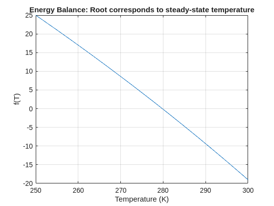
% Use fzero with an interval that brackets the root
T_eq = fzero(f, [250 300]);
fprintf('Steady-state temperature: %.2f K\n', T_eq);
Don’t miss out on two incredible keynotes that will shape the future of engineering and innovation:
1️⃣What’s New in MATLAB and Simulink in 2025
Get an inside look at the latest features designed to supercharge your workflows:
- A redesigned MATLAB desktop with customizable sidebars, light/dark themes, and new panels for coding tasks
- MATLAB Copilot – your AI-powered assistant for learning, idea generation, and productivity
- Simulink upgrades, including an enhanced quick insert tool, auto-straightening signal lines, and new methods for Python integration
- New options to deploy AI models on Qualcomm and Infineon hardware
2️⃣Accelerating Software-Defined Vehicles with Model-Based Design
See how MathWorks + NXP are transforming embedded system development for next-gen vehicles:
- Vehicle electrification example powered by MATLAB, Simulink, and NXP tools
- End-to-end workflow: modeling → validation → code generation → hardware deployment → real-time cloud monitoring
📅 When: November 13
💡Why Join? Stay ahead with cutting-edge tools, workflows, and insights from industry leaders.
The Cody Contest 2025 is underway, and it includes a super creative problem group which many of us have found fascinating. The central theme of the problems, expertly curated by @Matt Tearle, humorously revolves around the whims of the capricious dictator Lord Ned, as he goes out of his way to complicate the lives of his subjects and visitors alike. We cannot judge whether or not there's any truth to the rumors behind all the inside jokes, but it's obvious that the team had a lot of fun creating these; and we had even more fun solving them.
Today I want to showcase a way of graphically solving and visualizing one of those problems which I found very elegant, The Bridges of Nedsburg.
To briefly reiterate the problem, the number of islands and the arrangement of bridges of the city of Nedsburg are constantly changing. Lord Ned has decided to take advantage of this by charging visitors with an increasingly expensive n-bridge pass which allows them to cross up to n bridges in one journey. Given the Connectivity Matrix C, we are tasked with calculating the minimum n needed so that there is a path from every island to every other island in n steps or fewer.
Matt kindly provided us with some useful bit of math in the description detailing how to calculate the way to get from one island to another in an number of m steps. However, he has also hidden an alternative path to the solution in plain sight, in one of the graphs he provided. This involves the extremely useful and versatile class digraph, representing directed graphs, which have directional edges connecting the nodes. Here's some further great documentation and other cool resources on the topic for those who are interested in learning more about it:
Let's start using this class to explore a graphical solution to Lord Ned's conundrum. We will use the unit tests included in the problem to visualize the solution. We can retrieve the connectivity matrix for each case using the following function:
function C = getConnectivityMatrix(unit_test)
% Number of islands and bridge arrangement
switch unit_test
case 1
m = 3; idx = [3;4;8];
case 2
m = 3; idx = [3;4;7;8];
case 3
m = 4; idx = [2;7;8;10;13];
case 4
m = 4; idx = [4;5;7;8;9;14];
case 5
m = 5; idx = [5;8;11;12;14;18;22;23];
case 6
m = 5; idx = [2;5;8;14;20;21;24];
case 7
m = 6; idx = [3;4;7;11;18;23;24;26;30;32];
case 8
m = 6; idx = [3;11;12;13;18;19;28;32];
case 9
m = 7; idx = [3;4;6;8;13;14;20;21;23;31;36;47];
case 10
m = 7; idx = [4;11;13;14;19;22;23;26;28;30;34;35;37;38;45];
case 11
m = 8; idx = [2;4;5;6;8;12;13;17;27;39;44;48;54;58;60;62];
case 12
m = 8; idx = [3;9;12;20;24;29;30;31;33;44;48;50;53;54;58];
case 13
m = 9; idx = [8;9;10;14;15;22;25;26;29;33;36;42;44;47;48;50;53;54;55;67;80];
case 14
m = 9; idx = [8;10;22;32;37;40;43;45;47;53;56;57;62;64;69;70;73;77;79];
case 15
m = 10; idx = [2;5;8;13;16;20;24;27;28;36;43;49;53;62;71;75;77;83;86;87;95];
case 16
m = 10; idx = [4;9;14;21;22;35;37;38;44;47;50;51;53;55;59;61;63;66;69;76;77;84;85;86;90;97];
end
C = zeros(m);
C(idx) = 1;
end
The case in the example refers to unit test case 2.
unit_test = 2;
C = getConnectivityMatrix(unit_test);
disp(C)
D = digraph(C);
figure
p = plot(D,'LineWidth',1.5,'ArrowSize',10);
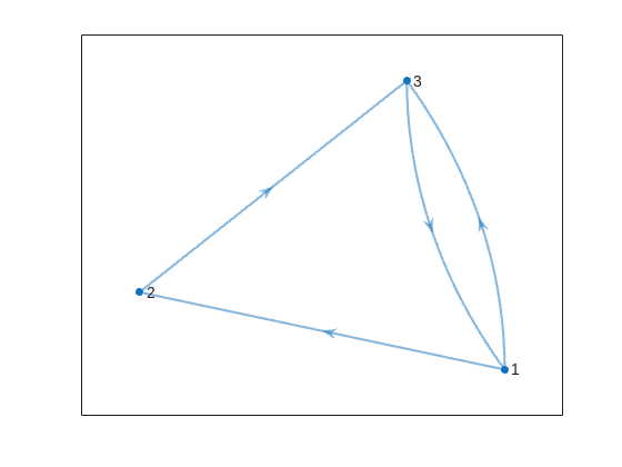
This is the same as the graph provided in the example. Another very useful method of digraph is shortestpath. This allows us to calculate the path and distance from one single node to another. For example:
% Path and distance from node 1 to node 2
[path12,dist12] = shortestpath(D,1,2);
fprintf('The shortest path from island %d to island %d is: %s. The minimum number of steps is: n = %d\n', 1, 2, join(string(path12), ' -> '),dist12)
% Path and distance from node 2 to node 1
[path21,dist21] = shortestpath(D,2,1);
fprintf('The shortest path from island %d to island %d is: %s. The minimum number of steps is: n = %d\n', 2, 1, join(string(path21), ' -> '),dist21)
figure
p = plot(D,'LineWidth',1.5,'ArrowSize',10);
highlight(p,path12,'EdgeColor','r','NodeColor','r','LineWidth',2)
highlight(p,path21,'EdgeColor',[0 0.8 0],'LineWidth',2)

But that's not all! digraph can also provide us with a matrix of the distances d, i.e. the steps needed to travel from island i to island j, where i and j are the rows and columns of d respectively. This is accomplished by using its distances method. The distance matrix can be visualized as:
d = distances(D);
figure
% Using pcolor w/ appending matrix workaround for convenience
pcolor([d,d(:,end);d(end,:),d(end,end)])
% Alternatively you can use imagesc(d), but you'll have to recreate the grid manually
axis square
set(gca,'YDir','reverse','XTick',[],'YTick',[])
[X,Y] = meshgrid(1:height(d));
text(X(:)+0.5,Y(:)+0.5,string(d(:)),'FontSize',11)
colormap(interp1(linspace(0,1,4), [1 1 1; 0.7 0.9 1; 0.6 0.7 1; 1 0.3 0.3], linspace(0,1,8)))
clim([-0.5 7+0.5])
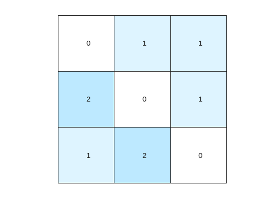
This confirms what we saw before, i.e. you need 1 step to go from island 1 to island 2, but 2 steps for vice versa. It also confirms that the minimum number of steps n that you need to buy the pass for is 2 (which also occurs for traveling from island 3 to island 2). As it's not the point of the post to give the full solution to the problem but rather present the graphical way of visualizing it I will not include the code of how to calculate this, but I'm sure that by now it's reduced to a trivial problem which you have already figured out how to solve.
That being said, now that we have the distance matrix, let's continue with the visualizations. First, let's plot the corresponding paths for each of these combinations:
figure
tiledlayout(size(C,1),size(C,2),'TileSpacing','tight','Padding','tight');
for i = 1:size(C,1)
for j = 1:size(C,2)
nexttile
p = plot(D,'ArrowSize',10);
highlight(p,shortestpath(D,i,j),'EdgeColor','r','NodeColor','r','LineWidth',2)
lims = axis;
text(lims(1)+diff(lims(1:2))*0.05,lims(3)+diff(lims(3:4))*0.9,sprintf('n = %d',d(i,j)))
end
end

This allows us to go from the distance matrix to visualizing the paths and number of steps for each corresponding case. Things are rather simple for this 3-island example case, but evil Lord Ned is just getting started. Let's now try to solve the problem for all provided unit test cases:
% Cell array of connectivity matrices
C = arrayfun(@getConnectivityMatrix,1:16,'UniformOutput',false);
% Cell array of corresponding digraph objects
D = cellfun(@digraph,C,'UniformOutput',false);
% Cell array of corresponding distance matrices
d = cellfun(@distances,D,'UniformOutput',false);
% id of solutions: Provided as is to avoid handing out the code to the full solution
id = [2, 2, 9, 3, 4, 6, 16, 4, 44, 43, 33, 34, 7, 18, 39, 2];
First, let's plot the distance matrix for each case:
figure
tiledlayout('flow','TileSpacing','compact','Padding','compact');
% Vary this to plot different combinations of cases
plot_cases = 1:numel(C);
for i = plot_cases
nexttile
pcolor([d{i},d{i}(:,end);d{i}(end,:),d{i}(end,end)])
axis square
set(gca,'YDir','reverse','XTick',[],'YTick',[])
title(sprintf('Case %d',i),'FontWeight','normal','FontSize',8)
end
c = colorbar('Ticks',0:7,'TickLength',0,'Limits',[-0.5 7+0.5],'FontSize',8);
c.Layout.Tile = 'East';
c.Label.String = 'Number of Steps';
c.Label.FontSize = 8;
colormap(interp1(linspace(0,1,4), [1 1 1; 0.7 0.9 1; 0.6 0.7 1; 1 0.3 0.3], linspace(0,1,8)))
clim(findobj(gcf,'type','axes'),[-0.5 7+0.5])
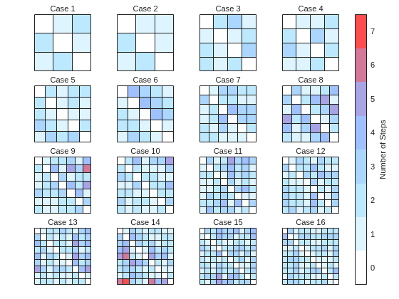
We immediately notice some inconsistencies, perhaps to be expected of the eccentric and cunning dictator. Things are pretty simple for the configurations with a small number of islands, but the minimum number of steps n can increase sharply and disproportionally to the additional number of islands. Cases 8 and 9 specifically have a particularly large n (relative to their grid dimensions), and case 14 has the largest n, almost double that of case 16 despite the fact that the latter has one extra island.
To visualize how this is possible, let's plot the path corresponding to the largest n for each case (though note that there might be multiple possible paths for each case):
figure
tiledlayout('flow','TileSpacing','tight','Padding','tight');
for i = plot_cases
nexttile
% Changing the layout to circular so we can better visualize the paths
p = plot(D{i},'ArrowSize',10,'Layout','Circle');
% Alternatively we could use the XData and YData properties if the positions of the islands were provided
axis([-1.5 1.5 -1.5 1.75])
[row,col] = ind2sub(size(d{i}),id(i));
highlight(p,shortestpath(D{i},row,col),'EdgeColor','r','NodeColor','r','LineWidth',2)
lims = axis;
text(lims(1)+diff(lims(1:2))*0.05,lims(3)+diff(lims(3:4))*0.9,sprintf('n = %d',d{i}(row,col)))
end
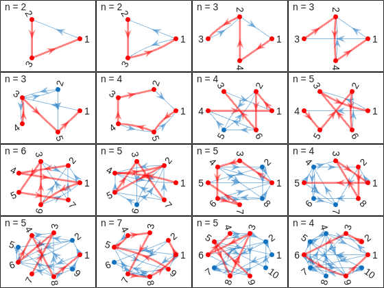
And busted! Unraveled! Exposed! Lord Ned has clearly been taking advantages of the tectonic forces by instructing his corrupt civil engineer lackeys to design the bridges to purposely force the visitors to go around in circles in order to drain them of their precious savings. In particular, for cases 8 and 9, he would have them go through every single island just to get from one island to another, whereas for case 14 they would have to visit 8 of the 9 islands just to get to their destination. If that's not diabolical then I don't know what is!
Ned jokes aside, I hope you enjoyed this contest just as much as I did, and that you found this article useful. I look forward to seeing more creative problems and solutions in the future.
Pure Matlab
82%
Simulink
18%
11 votes
Submit your questions about this work in the comment section below.