Sparse Model Basics
Model Objects
Use the sparss and mechss objects to represent sparse first-order and second-order
systems, respectively. Such sparse models arise from finite element analysis (FEA)
and are useful in fields like structural analysis, fluid flow, heat transfer and
electromagnetics. FEA involves analyzing a problem using finite element method (FEM)
where a large system is subdivided into numerous, smaller components or finite
elements (FE) which are then analyzed separately. These numerous components when
combined together result in large sparse models which are computationally expensive
and inefficient to be represented by traditional dense model objects like ss.
Sparse matrices provide efficient storage of double or logical data that has a large percentage of zeros. While full (or dense) matrices store every single element in memory regardless of value, sparse matrices store only the nonzero elements and their row indices. For this reason, using sparse matrices can significantly reduce the amount of memory required for data storage. For more information, see Computational Advantages of Sparse Matrices.
The following table illustrates the types of sparse models that can be represented:
| Model Type | Mathematical Representation | Model Object |
|---|---|---|
| Continuous-time sparse first-order model |
| sparss |
| Discrete-time sparse first-order model |
| sparss |
| Continuous-time sparse second-order model |
| mechss |
| Discrete-time sparse second-order model |
| mechss |
You can use sparssdata and mechssdata to access the model matrices in sparse form. You can also
use the spy
command to visualize the sparsity of both first-order and second-order model
matrices.
You can also convert any non-FRD model into a sparss or a mechss object respectively. Conversely, you can use the full
command to convert sparse models to dense storage ss. Converting to dense storage is
not recommended for large sparse models as it result in high memory usage and poor
performance.
Combining Sparse Models
Signal-Based Connections
All standard signal-based connections listed under Model Interconnection are supported for sparse model objects. Interconnecting models using signals allows you to construct models for control systems. You can conceptualize your control system as a block diagram containing multiple interconnected components, such as a plant and a controller connected in a feedback configuration. Using model arithmetic or interconnection commands, you combine models of each of these components into a single model representing the entire block diagram.
In series and feedback connections of sparss models, eliminating the internal signals can lead to
undesirable fill-in in the A matrix. To prevent this, the
software eliminates only those signals that do not affect the sparsity of
A and adds the remaining signals to the state vector. In
general, this produces a differential algebraic equation (DAE) model of the
interconnection where the A matrix has a block arrow
structure as depicted in the following figure:
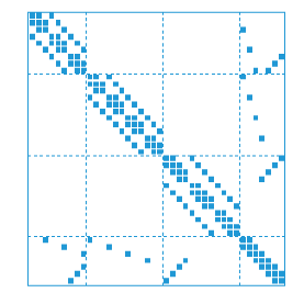
Here, each diagonal block is a sub-component of the sparse model. The last row
and column combines the Interface and
Signal groups to capture all couplings and connections
between components.
The same rules apply to second-order mechss model objects. You can use showStateInfo to print a summary of the state vector partition
into components, interfaces, and signals
Use the xsort command to sort states based on state partition. In the
sorted model, all components appear first, followed by the interfaces, and then
followed by a single group of all internal signals.
Physical Coupling
You can use the addInterface and assemble functions to specify physical couplings between the
components of sparss and mechss models. These functions model the coupling at the
interface using additional inputs and outputs. In general, you can represent
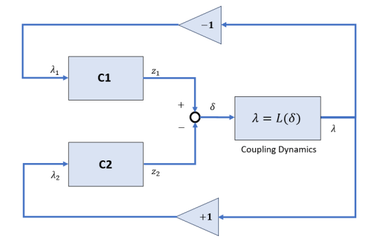
physical couplings in a block diagram form as shown in the following figure. The
coupling is characterized by the "Coupling Dynamics" block mapping
δ = z1 −
z2 (collocation gap) to the
internal forces λ. Here,
z1 and
z2 denote the positions on
each part of the nodes being coupled together.
Using Control System Toolbox™, you can perform the following types of couplings between state-space models.
Rigid couplings, which correspond to δ = 0 and λ determined by the balance of forces. In this type of coupling, the positions, z1 and z2 match exactly (collocation) as if the two parts were welded together.
Compliant couplings, where . Here the coupling is modeled as a spring-damper connection and the two parts can move with respect to each other.
Generalized coupling, where λ = Q(s)δ. Here, you obtain λ as the output of a linear system driven by the gap δ. This can be used to model more complex coupling dynamics.
For more information, see addInterface, assemble, and Rigid Assembly of Model Components.
Combining Models of Different Types
The following precedence rules apply when combining models of different types:
Combining sparse models with FRD models yields an
frdmodel objectCombining sparse models with any non-FRD model like
tf,ss, andzpkyields a sparse model objectCombining
sparssandmechssmodels yields amechssmodel object.Currently, sparse models cannot be combined with generalized or uncertain models,
genssanduss(Robust Control Toolbox).
For examples, see the mechss reference page.
Time-Domain Analysis
All standard time-domain analysis functions listed under Time and Frequency Domain Analysis are supported for sparss and mechss model objects.
You must specify a final time or time vector when using time-domain response functions for sparse models. For example:
tf = 10;
step(sys,tf)

t = 0:0.001:1;
initial(sys,x0,t)
The time response functions rely on custom fixed-step DAE solvers that have been
developed especially for large-scale sparse models. You can configure the DAE solver
type and enable parallel computing by using the SolverOptions
property of the sparss and mechss model objects. Parallel computing can be used to accelerate
step or impulse response simulation for
multi-input models as the response for each input channel is simulated in parallel.
Enabling parallel computing requires a Parallel Computing Toolbox™ license.
The available solver options are outlined in the table below:
| DAE Solver | Description | Usage |
|---|---|---|
'trbdf2'[2] | Fixed step solver with accuracy of o(h^2),
where h is the step size.
'trbdf2' is 50% more computationally
expensive than 'hht'. This is the default DAE
solver option for both sparss and mechss models. | Available for both sparss and mechss models. |
'trbdf3' | Fixed step solver with accuracy of o(h^3).
'trbdf3' is 50% more computationally
expensive than 'trbdf2'. | Available for both sparss and mechss models. |
'hht'[1] | Fixed step solver with accuracy of o(h^2),
where h is the step size.
'hht' is the fastest but can run into
difficulties with high initial acceleration like the impulse
response of a system. | Available for mechss models only. |
To enable parallel computing and solver selection, use the following syntax:
sys.SolverOptions.UseParallel = true;
sys.SolverOptions.DAESolver = 'trbdf3';
For an example, see Linear Analysis of Cantilever Beam.
Frequency-Domain Analysis
All standard frequency-domain analysis functions listed under Time and Frequency Domain Analysis are supported for sparss and mechss model objects. For frequency response computations, enabling
parallel computing speeds the response computation by distributing the set of
frequencies across available workers. Enabling parallel computing requires a
Parallel Computing Toolbox license.
You must specify a frequency vector when using frequency response functions for sparse models. For example:
w = logspace(0,8,1000);
bode(sys,w)
sigma(sys,w)
For an example, see Linear Analysis of Cantilever Beam.
Continuous and Discrete Conversions
You can convert between continuous-time and discrete-time, and resample sparss models using c2d, d2c and d2d. The following table outlines
the available methods for sparss models:
| Method | Description | Usage |
|---|---|---|
'tustin' | Bilinear Tustin approximation | Available with c2d, d2c and
d2d
functions. |
'damped' | Damped Tustin approximation based on
TRBDF2[2] formula. This method provides damping at infinity in contrast
to the 'tustin' method, that is, the high
frequency dynamics are filtered out and do not contribute to an
accumulation of modes near z = -1 in the
discrete model (a source of numerical instability). | Available with c2d
only. |
You can convert between continuous-time and
discrete-time, and resample mechss models using c2d, d2c and d2d with the
'tustin' method. The 'tustin' method
computes the second-order form of the Tustin discretization. This is equivalent to
applying Tustin to the first-order sparss equivalent of the
mechss model. This form is more favorable to modal
approximation since it preserves symmetry. (since R2024a)
Sparse Linearization
Linearize Simulink Model
You can obtain a sparse linearized model from a Simulink® model when a Descriptor State-Space (Simulink) or Sparse Second Order block is present.
The Sparse Second Order block is configured to always linearize to a
mechssmodel. As a result, the overall linearized model is a second-order sparse model when this block is present.Check the Linearize to sparse model option in the Descriptor State-Space (Simulink) block to linearize to a
sparssmodel. You can also achieve this by setting theLinearizerToSparseparameter to'on'in the Descriptor State-Space (Simulink). By default, the Linearize to sparse model box is unchecked and theLinearizerToSparseis'off'. The block-levelLinearizeToSparsesetting is ignored when you specify a replacement for the block, either with theSCDBlockLinearizationSpecificationblock parameter, or theblocksubinput tolinearize(Simulink Control Design).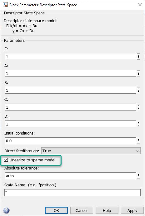
This linearization workflow requires Simulink Control Design™ software.
For an example, see Linearize Simulink Model to a Sparse Second-Order Model Object.
Linearize Structural or Thermal PDE Model
You can obtain a sparse linearized model from a structural or a thermal PDE
model by using the linearize (Partial Differential Equation Toolbox) function.
For a structural analysis model,
linearizeextracts amechssmodel.For a thermal analysis model,
linearizeextracts asparssmodel.
Use linearizeInput (Partial Differential Equation Toolbox) to specify the inputs of the linearized model in
terms of boundary conditions, loads, or internal heat sources in the PDE model.
Use linearizeOutput (Partial Differential Equation Toolbox) to specify the outputs of the linearized model
in terms of regions of the geometry, such as cells (for 3-D geometries only),
faces, edges, or vertices.
This linearization workflow requires Partial Differential Equation Toolbox™ software.
For examples, see Linear Analysis of Cantilever Beam and Linear Analysis of Tuning Fork.
Model Order Reduction
Since R2023b
To compute low-order approximations of sparse state-space models, use the
reducespec function. reducespec is the entry
point for model order reduction workflows in Control System Toolbox software. For the full workflow, see Task-Based Model Order Reduction Workflow.
The software supports sparse model order reduction using these methods.
Balanced truncation — Obtain low-order approximation by discarding states with low contribution.
Modal truncation — Obtain low-order approximation by discarding undesired modes.
Proper orthogonal decomposition — Perform an approximate balanced truncation using simulation data to compute and extract the dominant modes (principal components) of the state vector. (since R2025a)
Frequency response fitting — Fit low-order models to the frequency response data of large sparse state-space models. (since R2025a)
Zero-pole truncation — Obtain a zero-pole-gain approximation of sparse state-space models in a desired low-frequency band (since R2025a)
For examples, see SparseBalancedTruncation, SparseModalTruncation, ProperOrthogonalDecomposition, FrequencyResponseFitting, and SparseZeroPoleTruncation.
Additionally, you can use tf and zpk to obtain a truncated
tf or zpk model approximation of the
original sparse model in a specific low-frequency band. (since R2025a)
Other Supported Functionality
Additionally, the following functionality is currently supported for sparse models:
Low-frequency gain computation using
dcgainInverting models using
invImplicit-explicit relation conversions using
imp2expPadé approximations using
padeInput, output and internal delay specification
I/O selection and indexing
Compute a subset of poles, damping, natural frequency, and check stability in a specified frequency band using
pole,damp, andisstable. (since R2025a)
Limitations
The following operations are currently not supported for sparse models:
Stability margin computation
Compensator design and tuning
You can use the full
command to convert small sparse models to dense storage ss to perform the above
operations. Converting to dense storage is not recommended for large sparse models
as it may saturate available memory and cause severe performance degradation.
The following limitations exist for sparse linearization:
Sparse linearization is incompatible with block substitutions involving tunable or uncertain models. The Linearize to sparse model option should be unchecked when trying to linearize to
genssoruss(Robust Control Toolbox) models.Snapshot linearization may not work when the Descriptor State-Space (Simulink) or Sparse Second Order block is present. Since snapshot linearization requires simulation, the simulation capabilities are currently limited for the Descriptor State-Space (Simulink) and Sparse Second Order blocks.
References
[1] H. Hilber, T. Hughes & R. Taylor. " Improved numerical dissipation for time integration algorithms in structural dynamics." Earthquake Engineering and Structural Dynamics, vol. 5, no. 3, pp. 283-292, 1977.
[2] M. Hosea and L. Shampine. "Analysis and implementation of TR-BDF2." Applied Numerical Mathematics, vol. 20, no. 1-2, pp. 21-37, 1996.
See Also
sparss | mechss | showStateInfo | getx0 | full | sparssdata | mechssdata | xsort | interface | spy | Descriptor
State-Space (Simulink) | Sparse Second
Order