networkDistributionDiscriminator

Deep learning distribution discriminator

Since R2023a

Syntax

discriminator = networkDistributionDiscriminator(net,XID,XOOD,method)

discriminator = networkDistributionDiscriminator(net,XID,[],method)

discriminator = networkDistributionDiscriminator(net,[],XOOD,method)

discriminator = networkDistributionDiscriminator(___,Name=Value)

Description

discriminator = networkDistributionDiscriminator(net,XID,XOOD,method) returns a distribution discriminator using the method specified by method.

You can use the discriminator to classify observations as in-distribution (ID) and out-of-distribution (OOD). OOD data refers to data that is sufficiently different from the data you use to train the network, which can cause the network to behave unexpectedly. For more information, see In-Distribution and Out-of-Distribution Data.

The networkDistributionDiscriminator function first finds distribution confidence scores using the method you specify in method. The function then finds a threshold that best separates the ID and OOD distribution confidence scores. You can classify any observation with a score below the threshold as OOD. For more information about how the function computes the threshold, see Algorithms. You can find the threshold using a set of ID data, a set of OOD data, or both.

To determine whether new data is ID or OOD, pass discriminator as an input to the isInNetworkDistribution function.

To find the distribution confidence scores, pass discriminator as an input to the distributionScores function. For more information about distribution confidence scores, see Distribution Confidence Scores.

discriminator = networkDistributionDiscriminator(net,XID,[],method) returns a distribution discriminator using only the ID data. The Threshold property of discriminator contains the threshold such that the discriminator attains a true positive rate greater than the value of the TruePositiveGoal name-value argument. For more information, see Algorithms.

discriminator = networkDistributionDiscriminator(net,[],XOOD,method) returns a distribution discriminator using only the OOD data. The Threshold property of discriminator contains the threshold such that the discriminator attains a false positive rate less than the value of the FalsePositiveGoal name-value argument. For more information, see Algorithms.

discriminator = networkDistributionDiscriminator(___,Name=Value) returns a discriminator with additional options specified by one or more name-value arguments.

Examples

Create Distribution Discriminator Using In- and Out-of-Distribution Data

Load a pretrained classification network.

load("digitsClassificationMLPNet.mat");

Load ID data. Convert the data to a dlarray object.

XID = digitTrain4DArrayData;
XID = dlarray(XID,"SSCB");

Modify the ID training data to create an OOD set.

XOOD = XID*0.3 + 0.1;

Create a discriminator. The function finds the threshold that best separates the two distributions of data by maximizing the true positive rate and minimizing the false positive rate.

method = "baseline";
discriminator = networkDistributionDiscriminator(net,XID,XOOD,method)

discriminator = 
  BaselineDistributionDiscriminator with properties:

       Method: "baseline"
      Network: [1x1 dlnetwork]
    Threshold: 0.9743

Create Distribution Discriminator Using Only In-Distribution Data

Load a pretrained classification network.

load("digitsClassificationMLPNet.mat");

Load ID data. Convert the data to a dlarray object.

XID = digitTrain4DArrayData;
XID = dlarray(XID,"SSCB");

Create a discriminator using only the ID data. Set the method to "energy" with a temperature of 10. Specify the true positive goal as 0.975. To specify the true positive goal, you must specify ID data and not specify the false positive goal.

method = "energy";
discriminator = networkDistributionDiscriminator(net,XID,[],method, ...
    Temperature=10, ...
    TruePositiveGoal=0.975)

discriminator = 
  EnergyDistributionDiscriminator with properties:

         Method: "energy"
        Network: [1x1 dlnetwork]
    Temperature: 10
      Threshold: 23.5541

Create Distribution Discriminator Using Only Out-of-Distribution Data

Load a pretrained classification network.

load("digitsClassificationMLPNet.mat");

Create OOD data. In this example, the OOD data is 1000 images of random noise. Each image is 28-by-28 pixels, the same size as the input to the network. Convert the data to a dlarray object.

XOOD = rand([28 28 1 1000]);
XOOD = dlarray(XOOD,"SSCB");

Create a discriminator. Specify the false positive goal as 0.025. To specify the false positive goal, you must specify OOD data and not specify the true positive goal.

method = "baseline";
discriminator = networkDistributionDiscriminator(net,[],XOOD,method, ...
    FalsePositiveGoal=0.025)

discriminator = 
  BaselineDistributionDiscriminator with properties:

       Method: "baseline"
      Network: [1x1 dlnetwork]
    Threshold: 0.9998

Create Distribution Discriminator for Regression Network

Load a pretrained regression network.

load("digitsRegressionMLPNet.mat")

Load ID data. Convert the data to a dlarray object.

XID = digitTrain4DArrayData;
XID = dlarray(XID,"SSCB");

Modify the ID training data to create an OOD set.

XOOD = XID*0.3 + 0.1;

Create a discriminator. For regression tasks, set the method to "hbos". When using the HBOS method, you can specify additional options. Set the variance cutoff to 0.0001 and use the penultimate layer to compute the HBOS distribution scores.

method = "hbos";
discriminator = networkDistributionDiscriminator(net,XID,XOOD,method, ...
    VarianceCutoff=0.0001, ...
    LayerNames="relu_2")

discriminator = 
  HBOSDistributionDiscriminator with properties:

            Method: "hbos"
           Network: [1×1 dlnetwork]
        LayerNames: "relu_2"
    VarianceCutoff: 1.0000e-04
         Threshold: -54.1244

Assess Performance of Distribution Discriminator

Load a pretrained classification network.

load('digitsClassificationMLPNet.mat');

Load ID data. Convert the data to a dlarray object and count the number of observations.

XID = digitTrain4DArrayData;
XID = dlarray(XID,"SSCB");
numObservations = size(XID,4);

Modify the ID training data to create an OOD set.

XOOD = XID*0.3 + 0.1;

Create a discriminator. The function finds the threshold that best separates the two distributions of data.

method = "baseline";
discriminator = networkDistributionDiscriminator(net,XID,XOOD,method);

Test the discriminator on the ID and OOD data using the isInNetworkDistribution function. The isInNetworkDistribution function returns a logical array indicating which observations are ID and which observations are OOD.

tfID = isInNetworkDistribution(discriminator,XID);
tfOOD = isInNetworkDistribution(discriminator,XOOD);

Calculate the accuracy for the ID and OOD observations.

accuracyID = sum(tfID == 1)/numel(tfID)

accuracyID = 0.9856

accuracyOOD = sum(tfOOD == 0)/numel(tfOOD)

accuracyOOD = 0.9402

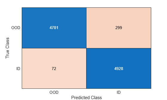
Plot the confusion chart for the ID and OOD data.

trueDataLabels = [
    repelem("In-Distribution",numObservations), ...
    repelem("Out-of-Distribution",numObservations)];

predDataLabelsID = repelem("Out-of-Distribution",numObservations);
predDataLabelsID(tfID == 1) = "In-Distribution";

predDataLabelsOOD = repelem("Out-of-Distribution",numObservations);
predDataLabelsOOD(tfOOD == 1) = "In-Distribution";

predDataLabels = [predDataLabelsID,predDataLabelsOOD];

confusionchart(trueDataLabels,predDataLabels)

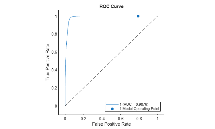
Use the distributionScores function to find the distribution scores for the ID and OOD data.

scoresID = distributionScores(discriminator,XID);
scoresOOD = distributionScores(discriminator,XOOD);
scores = [scoresID',scoresOOD'];

Use rocmetrics to plot a ROC curve to show how well the model is at separating the data into ID and OOD.

rocObj = rocmetrics(trueDataLabels,scores,"In-Distribution");
plot(rocObj)

Create Distribution Discriminator Using Mini-Batches

Load a pretrained classification network.

load("digitsClassificationMLPNet.mat");

Load the digit sample data and create an image datastore. The imageDatastore function automatically labels the images based on folder names.

digitDatasetPath = fullfile(matlabroot,'toolbox','nnet','nndemos', ...
    'nndatasets','DigitDataset');
imds = imageDatastore(digitDatasetPath, ...
    'IncludeSubfolders',true,'LabelSource','foldernames');

Create the minibatchqueue object.

• Specify a mini-batch size of 64.

• Preprocess the mini-batches using the preprocessMiniBatch function, listed at the end of this example.

• Convert the output to a dlarray object.

• Specify that the output data has format "SSCB" (spatial, spatial, channel, batch).

mbq = minibatchqueue(imds, ...
    MiniBatchSize=64, ...
    MiniBatchFcn=@preprocessMiniBatch, ...
    OutputAsDlarray=true, ...
    MiniBatchFormat="SSCB");

Create a discriminator using the minibatchqueue object containing ID data. Set the method to "baseline" and the VerbosityLevel to "detailed".

method = "baseline";
discriminator = networkDistributionDiscriminator(net,mbq,[],method,VerbosityLevel="detailed");

Processing in-distribution data:
Computing distribution scores...
..........   ..........   ..........   ..........   .......... (50 mini-batches)
..........   ..........   ..........   ..........   .......... (100 mini-batches)
..........   ..........   ..........   ..........   .......... (150 mini-batches)
.......                                                        (157 mini-batches)
Done.
Computing threshold...Done.

Mini-Batch Preprocessing Function

The preprocessMiniBatch function preprocesses the data using the following steps:

1. Extract the image data from the incoming cell array and concatenate the data into a numeric array.

2. Rescale the images to the range [0 1].

function X = preprocessMiniBatch(dataX)
X = cat(4,dataX{1:end});
X = rescale(X,InputMin=0,InputMax=1);
end

Input Arguments

net — Neural network

dlnetwork object

Neural network, specified as a dlnetwork object.

XID — In-distribution data

formatted dlarray object | minibatchqueue object | []

In-distribution (ID) data, specified as a formatted dlarray object, a minibatchqueue object that returns formatted dlarray objects, or []. For more information about dlarray formats, see the fmt input argument of dlarray.

At least one of the XID and XOOD input arguments must be nonempty.

For more information about ID and OOD data, see In-Distribution and Out-of-Distribution Data.

XOOD — Out-of-distribution data

formatted dlarray object | minibatchqueue object | []

Out-of-distribution (OOD) data, specified as a formatted dlarray object, a minibatchqueue object that returns formatted dlarray objects, or []. For more information about dlarray formats, see the fmt input argument of dlarray.

At least one of the XID and XOOD input arguments must be nonempty.

For more information about ID and OOD data, see In-Distribution and Out-of-Distribution Data.

method — Method for computing distribution confidence scores

"baseline" | "odin" | "energy" | "hbos"

Method for computing the distribution confidence scores, specified as one of these values:

• "baseline" — Use maximum softmax activations as the distribution confidence scores [1]. This method creates a BaselineDistributionDiscriminator object.

• "odin" — Use rescaled softmax activations as distribution confidence scores (also known as the ODIN method) [2]. Set the scale by specifying the Temperature name-value argument. This method creates an ODINDistributionDiscriminator object.

• "energy" — Use scaled, energy-based distribution confidence scores [3]. Set the scale by specifying the Temperature name-value argument. This method creates an EnergyDistributionDiscriminator object.

• "hbos" — Use histogram-based outlier scores (also known as the HBOS method) [4] as distribution confidence scores. The function computes the scores by constructing histograms for the principal component features for each layer that you specify in the LayerNames name-value argument. Use the VarianceCutoff name-value argument to control the number of principal component features the software uses. To use this method, XID must be nonempty. This method creates a HBOSDistributionDiscriminator object.

For more information about each method, see Distribution Confidence Scores.

Note

Specifying method as "baseline", "odin", or "energy" is valid only for single-output networks with a softmax layer as the final layer. For example, specifying net as a single-output classification network. You can specify method as "hbos" for any network.

Data Types: char | string

Name-Value Arguments

Specify optional pairs of arguments as Name1=Value1,...,NameN=ValueN, where Name is the argument name and Value is the corresponding value. Name-value arguments must appear after other arguments, but the order of the pairs does not matter.

Before R2021a, use commas to separate each name and value, and enclose Name in quotes.

Example: TruePositiveGoal=0.99,Temperature=10

TruePositiveGoal — True positive goal

0.95 (default) | scalar in the range [0, 1]

True positive goal, specified as a scalar in the range [0, 1]. The software returns the threshold that correctly classifies at least this proportion of the ID data as ID.

Dependency

If you specify a true positive goal, then XID must be nonempty and you cannot specify FalsePositiveGoal. If you specify a nonempty XOOD value, then the software uses only XID to compute the threshold.

If you do not specify the TruePositiveGoal and FalsePositiveGoal name-value arguments and provide nonempty XID and XOOD values, then the function does not use the default values and instead optimizes over the true positive rate and false positive rate to find the optimal threshold. For more information, see Algorithms.

Data Types: single | double | int8 | int16 | int32 | int64 | uint8 | uint16 | uint32 | uint64

FalsePositiveGoal — False positive goal

0.05 (default) | scalar in the range [0, 1]

False positive goal, specified as a scalar in the range [0, 1]. The software returns the threshold that incorrectly classifies at most this proportion of the OOD data as ID.

Dependency

If you specify a false positive goal, then XOOD must be nonempty and you must not specify TruePositiveGoal. If you specify a nonempty XID value, then the software uses only XOOD to compute the threshold.

If you do not specify the TruePositiveGoal and FalsePositiveGoal name-value arguments and provide nonempty XID and XOOD values, then the function does not use the default values and instead optimizes over the true positive rate and false positive rate to find the optimal threshold. For more information, see Algorithms.

Data Types: single | double | int8 | int16 | int32 | int64 | uint8 | uint16 | uint32 | uint64

Temperature — Temperature scaling

1 (default) | positive scalar

Temperature scaling for the ODIN and energy methods, specified as a positive scalar. The temperature controls the scaling of the softmax scores when the function computes the distribution confidence scores. For more information, see Distribution Confidence Scores.

Dependency

To enable this input, specify method as "odin" or "energy".

Data Types: single | double | int8 | int16 | int32 | int64 | uint8 | uint16 | uint32 | uint64

LayerNames — Layer names

string scalar | character vector | string array | cell array of character vectors

Layer names for the HBOS method, specified as a string scalar, character vector, string array, or cell array of character vectors. The default value is the first layer specified in the OutputNames property of net.

The software computes the distribution confidence scores using the principal components from all of the specified layers. For more information, see Density-Based Methods.

Note

To compute the histograms, the software must first compute the principal component features for each layer. Computing the principal components can be slow for layers with a large output size and can cause you to run out of memory. If you run out of memory, try specifying layers with a smaller output size. For more information, see Density-Based Methods.

Dependency

To enable this input, specify method as "hbos".

Data Types: char | string | cell

VarianceCutoff — Variance cutoff

1e-3 (default) | scalar in the range [0, 1]

Variance cutoff for the HBOS method, specified as a scalar in the range [0, 1].

The variance cutoff controls the number of principal component features that the software uses to compute the distribution confidence scores. Using a greater number of features takes more computation time. The closer the VarianceCutoff value is to 1, the fewer principal components the software uses to compute the scores. For more information, see Density-Based Methods.

Dependency

To enable this input, specify method as "hbos".

Data Types: single | double | int8 | int16 | int32 | int64 | uint8 | uint16 | uint32 | uint64

VerbosityLevel — Verbosity level

"off" (default) | "summary" | "detailed"

Verbosity level of the Command Window output, specified as one of these values:

• "off" — Do not display progress information.

• "summary" — Display a summary of the progress information.

• "detailed" — Display detailed information about the progress. This option prints the mini-batch progress. If you do not specify the input data as a minibatchqueue object, then the "detailed" and "summary" options print the same information.

Output Arguments

discriminator — Distribution discriminator

BaselineDistributionDiscriminator object | ODINDistributionDiscriminator object | EnergyDistributionDiscriminator object | HBOSDistributionDiscriminator object

Distribution discriminator, returned as a BaselineDistributionDiscriminator, ODINDistributionDiscriminator, EnergyDistributionDiscriminator, or HBOSDistributionDiscriminator object.

The function returns this output as a BaselineDistributionDiscriminator, ODINDistributionDiscriminator, EnergyDistributionDiscriminator, or HBOSDistributionDiscriminator object when you specify method as "baseline", "odin", "energy", or "hbos", respectively.

The Threshold property of discriminator contains the threshold for separating the ID and OOD data. To access the threshold value, call discriminator.Threshold.

More About

In-Distribution and Out-of-Distribution Data

In-distribution (ID) data refers to any data that you use to construct and train your model. Additionally, any data that is sufficiently similar to the training data is also said to be ID.

Out-of-distribution (OOD) data refers to data that is sufficiently different to the training data. For example, data collected in a different way, at a different time, under different conditions, or for a different task than the data on which the model was originally trained. Models can receive OOD data when you deploy them in an environment other than the one in which you train them. For example, suppose you train a model on clear X-ray images but then deploy the model on images taken with a lower-quality camera.

OOD data detection is important for assigning confidence to the predictions of a network. For more information, see OOD Data Detection.

OOD Data Detection

OOD data detection is a technique for assessing whether the inputs to a network are OOD. For methods that you apply after training, you can construct a discriminator which acts as an additional output of the trained network that classifies an observation as ID or OOD.

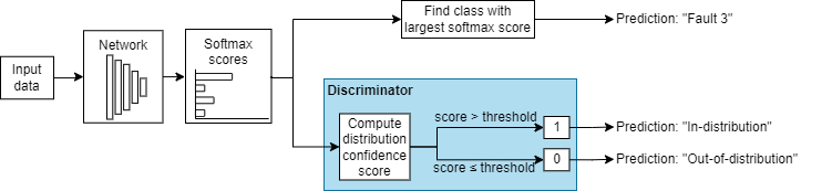
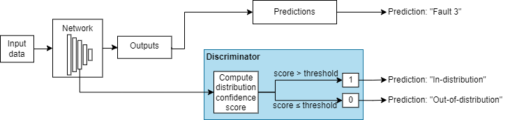
The discriminator works by finding a distribution confidence score for an input. You can then specify a threshold. If the score is less than or equal to that threshold, then the input is OOD. Two groups of metrics for computing distribution confidence scores are softmax-based and density-based methods. Softmax-based methods use the softmax layer to compute the scores. Density-based methods use the outputs of layers that you specify to compute the scores. For more information about how to compute distribution confidence scores, see Distribution Confidence Scores.

These images show how a discriminator acts as an additional output of a trained neural network.

Example Data Discriminators

Example of Softmax-Based Discriminator	Example of Density-Based Discriminator
For more information, see Softmax-Based Methods.	For more information, see Density-Based Methods.

Distribution Confidence Scores

Distribution confidence scores are metrics for classifying data as ID or OOD. If an input has a score less than or equal to a threshold value, then you can classify that input as OOD. You can use different techniques for finding the distribution confidence scores.

Softmax-Based Methods

ID data usually corresponds to a higher softmax output than OOD data[1]. Therefore, a method of defining distribution confidence scores is as a function of the softmax scores. These methods are called softmax-based methods. These methods only work for classification networks with a single softmax output.

Let a_i(X) be the input to the softmax layer for class i. The output of the softmax layer for class i is given by this equation:

$$P_i(X;T)=\frac{e^{a_i(X)/T}}{{\displaystyle \sum _{j=1}^C{e}^{a_j(X)/T}}},$$

where C is the number of classes and T is a temperature scaling. When the network predicts the class label of X, the temperature T is set to 1.

The baseline, ODIN, and energy methods each define distribution confidence scores as functions of the softmax input.

• The baseline method [1] uses the maximum of the unscaled output values of the softmax scores:

  $$\text{confidence}(X)=\underset{i}{\max }{P}_i(X;1).$$

• The out-of-distribution detector for neural networks (ODIN) method [2] uses the maximum of the scaled output of the softmax scores:

  $$\text{confidence}(X;T)=\underset{i}{\max }{P}_i(X;T)\text{, }T>0.$$

• The energy method [3] uses the scaled denominator of the softmax output:

  $$\begin{array}{l}\text{energy}(X;T)=-T\log \left({\displaystyle \sum _{j=1}^C{e}^{a_j(X)/T}}\right)\text{, }T>0\\ \text{confidence}(X;T)=-\text{energy}(X;T)\text{, }T>0.\end{array}$$

Density-Based Methods

Density-based methods compute the distribution scores by describing the underlying features learned by the network as probabilistic models. Observations falling into areas of low density correspond to OOD observations.

To model the distributions of the features, you can describe the density function for each feature using a histogram. This technique is based on the histogram-based outlier score (HBOS) method [4]. This method uses a data set of ID data, such as training data, to construct histograms representing the density distributions of the ID features. This method has three stages:

1. Find the principal component features for which to compute the distribution confidence scores:

   1. For each specified layer, find the activations using the n data set observations. Flatten the activations across all dimensions except the batch dimension.

   2. Compute the principal components of the flattened activations matrix. Normalize the eigenvalues such that the largest eigenvalue is 1 and corresponds to the principal component that carries the greatest variance through the layer. Denote the matrix of principal components for layer l by Q^(l).

      The principal components are linear combinations of the activations and represent the features that the software uses to compute the distribution scores. To compute the score, the software uses only the principal components whose eigenvalues are greater than the variance cutoff value σ.

      Note

      The HBOS algorithm assumes that the features are statistically independent. The principal component features are pairwise linearly independent but they can have nonlinear dependencies. To investigate feature dependencies, you can use functions such as corr (Statistics and Machine Learning Toolbox). For an example showing how to investigate feature dependence, see Out-of-Distribution Data Discriminator for YOLO v4 Object Detector. If the features are not statistically independent, then the algorithm can return poor results. Using multiple layers to compute the distribution scores can increase the number of statistically dependent features.

2. For each of the principal component features with an eigenvalue greater than σ, construct a histogram. For each histogram:

   1. Dynamically adjusts the width of the bins to create $$\sqrt{n}$$ bins of approximately equal area.

   2. Normalize the bins heights such that the largest height is 1.

3. Find the distribution score for an observation by summing the logarithmic height of the bin containing the observation for each of the feature histograms, over each of the layers.

   Let f^(l)(X) denote the output of layer l for input X. Use the principal components to project the output into a lower dimensional feature space using this equation: $${\widehat{f}}^{(l)}(X)={\left(Q^{(l)}\right)}^T{f}^{(l)}(X)$$.

   Compute the confidence score using this equation:

   $$\begin{array}{l}\text{HBOS}(X;\sigma )=-{\displaystyle \sum _{l=1}^L\left({\displaystyle \sum _{k=1}^{N^{(l)}(\sigma )}\text{log}\left({\text{hist}}_k\left({\widehat{f}}_k^{(l)}(X)\right)\right)}\right)},\\ \text{confidence}(X;\sigma )=-\text{HBOS}(X;\sigma ),\end{array}$$

   where N^(l)(σ) is the number of number of principal component with an eigenvalue less than σ and L is the number of layers. A larger score corresponds to an observation that lies in the areas of higher density. If the observation lies outside of the range of any of the histograms, then the bin height for those histograms is 0 and the confidence score is -Inf.

   Note

   The distribution scores depend on the properties of the data set used to construct the histograms [6].

Algorithms

The function creates a discriminator using the trained network. The discriminator behaves as an additional output of the network and classifies an observation as ID or OOD using a threshold. For more information, see OOD Data Detection.

To compute the distribution threshold, the function first computes the distribution confidence scores using the method that you specify in the method input argument. For more information, see Distribution Confidence Scores. The software then finds the threshold that best separates the scores of the ID and OOD data. To find the threshold, the software optimizes over these values:

• True positive goal — Number of ID observations that the discriminator correctly classifies as ID. To optimize for this value, the ID data XID must be nonempty and you must specify TruePositiveGoal. If you specify TruePositiveGoal as p, then the software finds the threshold above which the proportion of ID confidence scores is p. This process is equivalent to finding the 100(1-p)-th percentile for the ID confidence scores.

• False positive goal — Number of OOD observations that the discriminator incorrectly classifies as ID. To optimize for this value, the OOD data XOOD must be nonempty and you must specify FalsePositiveGoal. If you specify FalsePositiveGoal as p, then the software finds the threshold above which the proportion of OOD confidence scores is p. This process is equivalent to finding the 100p-th percentile for the OOD confidence scores.

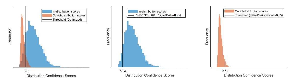
If you provide ID and OOD data and do not specify TruePositiveGoal or FalsePositiveGoal, then the software finds the threshold that maximizes the balanced accuracy $$\frac{1}{2}(TPR+(1-FPR))$$. If you provide only ID data, then the software optimizes using only TruePositiveGoal, whose default is 0.95. If you provide only OOD data, then the software optimizes using only FalsePositiveGoal, whose default is 0.05.

This figure illustrates the different thresholds that the software chooses if you optimize over both the true positive rate and false positive rate, just the true positive rate, or just the false positive rate.

References

[1] Shalev, Gal, Gabi Shalev, and Joseph Keshet. “A Baseline for Detecting Out-of-Distribution Examples in Image Captioning.” In Proceedings of the 30th ACM International Conference on Multimedia, 4175–84. Lisboa Portugal: ACM, 2022. https://doi.org/10.1145/3503161.3548340.

[2] Shiyu Liang, Yixuan Li, and R. Srikant, “Enhancing The Reliability of Out-of-distribution Image Detection in Neural Networks” arXiv:1706.02690 [cs.LG], August 30, 2020, http://arxiv.org/abs/1706.02690.

[3] Weitang Liu, Xiaoyun Wang, John D. Owens, and Yixuan Li, “Energy-based Out-of-distribution Detection” arXiv:2010.03759 [cs.LG], April 26, 2021, http://arxiv.org/abs/2010.03759.

[4] Markus Goldstein and Andreas Dengel. "Histogram-based outlier score (hbos): A fast unsupervised anomaly detection algorithm." KI-2012: poster and demo track 9 (2012).

[5] Jingkang Yang, Kaiyang Zhou, Yixuan Li, and Ziwei Liu, “Generalized Out-of-Distribution Detection: A Survey” August 3, 2022, http://arxiv.org/abs/2110.11334.

[6] Lee, Kimin, Kibok Lee, Honglak Lee, and Jinwoo Shin. “A Simple Unified Framework for Detecting Out-of-Distribution Samples and Adversarial Attacks.” arXiv, October 27, 2018. http://arxiv.org/abs/1807.03888.

Extended Capabilities

C/C++ Code Generation

Generate C and C++ code using MATLAB® Coder™.

Usage notes and limitations:

• To load a discriminator object for code generation, use the coder.loadNetworkDistributionDiscriminator function.

• Requires the MATLAB^® Coder™ Interface for Deep Learning support package. If this support package is not installed, use the Add-On Explorer. To open the Add-On Explorer, go to the MATLAB® Toolstrip and click Add-Ons > Get Add-Ons.

GPU Code Generation

Generate CUDA® code for NVIDIA® GPUs using GPU Coder™.

Usage notes and limitations:

• To load a discriminator object for code generation, use the coder.loadNetworkDistributionDiscriminator function.

• Requires the GPU Coder™ Interface for Deep Learning support package. If this support package is not installed, use the Add-On Explorer. To open the Add-On Explorer, go to the MATLAB® Toolstrip and click Add-Ons > Get Add-Ons.

GPU Arrays

Accelerate code by running on a graphics processing unit (GPU) using Parallel Computing Toolbox™.

Usage notes and limitations:

• This function runs on the GPU if its inputs meet either or both of these conditions:

  • Any values of the network learnable parameters are dlarray objects with underlying data of type gpuArray. To see the learnables for a network net, call net.Learnables.Value.

  • Any of the data is a dlarray object with underlying data of type gpuArray.

For more information, see Run MATLAB Functions on a GPU (Parallel Computing Toolbox).

Version History

Introduced in R2023a

R2024a: Use networks with multiple inputs

The networkDistributionDiscriminator function now support networks with multiple inputs.

R2023a: Display progress information (June 2023; Version 23.1.1)

Set the VerbosityLevel option to view progress information. The software displays progress information in the Command Window. You can set the VerbosityLevel to "off", "summary", or "detailed".

R2023a: Use minibatchqueue objects (June 2023; Version 23.1.1)

Detect out-of-distribution data using minibatchqueue objects. You can use minibatchequeue objects to create, preprocess, and manage mini-batches of data, and to automatically convert your data to a dlarray object.

R2023a: Code generation support (June 2023; Version 23.1.1)

Generate C or C++ code using MATLAB Coder or generate CUDA^® code for NVIDIA^® GPUs using GPU Coder. For more information, see coder.loadNetworkDistributionDiscriminator.