Georeference Sequence of Point Clouds for Scene Generation
This example shows how to register and stitch a sequence of point clouds and georeference the resulting registered point cloud by using GPS data.
You can use a combination of sensors to create a virtual scene that includes both a road network and static objects. For example, you can use a camera and GPS data to reconstruct a road network, while, using lidar data to recreate static scene objects such as buildings and trees. Alternatively, you can use the OpenStreetMap® live map service to reconstruct road networks. However you create your virtual road network, you must ensure that the data from various sensors and maps align within a consistent spatial coordinate system. A georeferenced point cloud ensures that the point locations within the point cloud correspond accurately with maps, such as an OpenStreetMap or RoadRunner HD Map.
Lidar sensors, in the context of automated driving, are typically mounted on an ego vehicle, and generate a sequence of point clouds. You must register and stitch the sequence of point clouds to reconstruct a 3-D scene represented by a single point cloud. For more information on how to register and stitch point clouds, see the 3-D Point Cloud Registration and Stitching example. To improve the accuracy of point cloud registration and stitching using an inertial navigation sensor (INS), see the Build a Map from Lidar Data Using SLAM example.
In this example, you:
Load and visualize the point cloud sequence data
Register and stitch a sequence of point clouds
Georeference the registered point cloud using GPS data
Validate the georeferenced point cloud
This example requires the Scenario Builder for Automated Driving Toolbox™ support package. Check if the support package is installed and, if not, install it using the Add-On Manager. For more information on installing support packages, see Get and Manage Add-Ons.
checkIfScenarioBuilderIsInstalled
Load and Visualize Point Cloud Sequence Data
Download a ZIP file containing a subset of sensor data from the PandaSet data set, and then unzip the file. This file contains data for a continuous sequence of 80 point clouds, images, and GPS data. However, this example uses the lidar and GPS data to create a georeferenced point cloud.
Note: The first latitude, longitude and altitude values in the GPS data must correspond to the origin of the first point cloud in the point cloud sequence.
tmpFolder = tempdir;
dataFilename = "PandasetData089.zip";
url = "https://ssd.mathworks.com/supportfiles/driving/data/" + dataFilename;
filePath = fullfile(tmpFolder,dataFilename);
if ~isfile(filePath)
    websave(filePath,url);
end

dataFolder = fullfile(tmpFolder,"PandasetData089");
mkdir(dataFolder)
Warning: Directory already exists.
unzip(filePath,dataFolder)
Extract the sequence of point clouds, GPS data, and lidar transformations from the downloaded PandaSet sensor data by using the helperLoadVehicleDataForGeoreferencing helper function, attached to this example as a supporting file. The lidar transformations are stored in the Attributes property of the lidarData and contains the rigidtform3d transformation that transforms the point cloud from sensor coordinates to world coordinates.
[lidarData, gpsData] = helperLoadVehicleDataForGeoReferencing(dataFolder);
Read and visualize the first point cloud in the point cloud array ptCldArray.
ptCldData = read(lidarData,RowIndices=1);
pcshow(ptCldData.PointClouds{1})
xlabel("X")
ylabel("Y")
zlabel("Z")
Notice that the point cloud does not follow the sensor coordinate system in Lidar Toolbox™. For more information, see Coordinate Systems in Lidar Toolbox (Lidar Toolbox). According to the sensor coordinate system in Lidar Toolbox, the x-axis is positive in the direction of movement of the ego vehicle, the y-axis is positive to the left of the direction of movement of the ego vehicle, and the z-axis is positive upward from the ground. However, for the lidar sensor frame of the PandaSet data set, the direction of movement of the ego vehicle is the positive y-axis, and the left of the direction of movement of the ego vehicle is the negative x-axis. Thus, you must apply a rotation of –90 degrees around the positive z-axis.
Specify helperRotatePointCloud helper function as PostProcessingFcn to read, to rotate the point clouds by –90 degrees around the positive z-axis.
ptCldData = read(lidarData,RowIndices=1,PostProcessingFcn=@helperRotatePointCloud);
Visualize the first transformed point cloud.
Verify that the ego vehicle is present at (0, 0) in xy-coordinates. The positive x-axis points forward from the ego vehicle and the positive y-axis points to the left of the ego vehicle.
pcshow(ptCldData.PointClouds{1})
xlabel("X")
ylabel("Y")
zlabel("Z")
Register and Stitch Sequence of Point Clouds
To compose a larger 3-D world scene, you can register and stitch a sequence of point clouds by using the iterative closest point (ICP) algorithm. Use the first point cloud to establish the reference coordinate system. Transform each subsequent point cloud to the reference coordinate system. For more information, see the 3-D Point Cloud Registration and Stitching example.
% Use the first point cloud as the reference point cloud and stitch all the point clouds.
ptCldSceneData = read(lidarData,RowIndices=1,PostProcessingFcn=@helperRotatePointCloud);
ptCldScene = ptCldSceneData.PointClouds{1};

for i = 2:lidarData.NumSamples

    pcFixed = read(lidarData,RowIndices=i-1,PostProcessingFcn=@helperRotatePointCloud);
    pcMoving = read(lidarData,RowIndices=i,PostProcessingFcn=@helperRotatePointCloud);

    % Preprocess the point cloud by downsampling with a box grid filter of
    % size 0.05 m.
    fixed = pcdownsample(pcFixed.PointClouds{1},"gridAverage",0.05);
    moving = pcdownsample(pcMoving.PointClouds{1},"gridAverage",0.05);

    % Apply the ICP registration algorithm. For each registration step after the first, use the
    % transformation estimated at the previous step as the initial
    % transformation.
    if i==2
        tform = pcregistericp(moving,fixed,Metric="planeToPlane");
        accumTform = tform;
    else
        tform = pcregistericp(moving,fixed,Metric="planeToPlane",InitialTransform=tform,Tolerance=[0.01 0.01]);
        accumTform = rigidtform3d(accumTform.A*tform.A);
    end

    % Transform the current moving point cloud to the reference coordinate system
    % defined by the first fixed point cloud.
    pcAligned = pctransform(pcMoving.PointClouds{1},accumTform);

    % Merge point clouds to create the complete scene.
    ptCldScene = pcmerge(ptCldScene,pcAligned,0.05);
end
Visualize the stitched 3-D point cloud that represents the complete scene.
Note: The terrestrial point cloud registration process builds a map of the scene traversed by the vehicle. Although the map might appear locally consistent with reference to the first point cloud in the sequence, you might observe a significant drift over the entire sequence. If you have the Inertial Measurement Unit (IMU) and GPS data for each point cloud in the sequence, you can use it to improve the performance of the point cloud registration. For more information, see the Build a Map from Lidar Data example.
pcshow(ptCldScene)
zoom(2)
title("Terrestrial Point Cloud: Complete Scene")
To check if the point cloud is a georeferenced point cloud, overlay the ego trajectory on the point cloud. Create trajectory from gpsData using trajectory function. Use the first latitude, longitude, and altitude values as the origin of the local coordinate system.
% Create a trajectory.
localOrigin = [gpsData.Latitude(1), gpsData.Longitude(1), gpsData.Altitude(1)];
traj = trajectory(gpsData,LocalOrigin=localOrigin);
View the point cloud and the overlaid ego vehicle trajectory. Observe that the point cloud does not align with the ego trajectory.
figHandle = plot(traj,Color="red",MarkerSize=10);
hold on
pcshow(ptCldScene,Parent=figHandle.CurrentAxes)
zoom(2)
title("Terrestrial Point Cloud: Complete Scene")
hold off

Georeference Registered Point Cloud Using GPS Data
To align the registered point cloud along the ego vehicle trajectory, you must georeference the point cloud.
Georeference the point cloud using GPS data by using the helperTransformPointCloud helper function, attached to this example as a supporting file. The helper function does not require time-synchronized data from lidar and GPS sensors. The latitude and longitude of the geographic coordinate system use the WGS84 standard that is commonly used by GPS receivers.
Note: Ensure that the first latitude, longitude, and altitude values in the GPS data correspond to the origin of the first point cloud in the loaded point cloud sequence.
[georeferencedPointCloud,localOrigin] = helperTransformPointCloud(ptCldScene,gpsData);
Validate Georeferenced Point Cloud
To validate whether the point cloud is georeferenced, overlay the ego trajectory on the point cloud and verify that the trajectory of the ego vehicle overlaps with the road in the point cloud. Note that georeference, which specifies the geographic origin of the georeferenced point cloud, is the first value each of latitude, longitude, and altitude from the extracted GPS data gpsData.
View the georeferenced point cloud and overlaid ego vehicle trajectory. Observe that the georeferenced point cloud aligns with the ego vehicle trajectory.
figHandle = plot(traj,Color="red",MarkerSize=10);
hold on
pcshow(georeferencedPointCloud,Parent=figHandle.CurrentAxes)
zoom(3)
title("Terrestrial Point Cloud: Complete Scene")
hold off

You also validate whether the point cloud is georeferenced using a map data. To validate, you must verify whether the locations of points in the georeferenced point cloud align with the locations of road boundaries in the associated OpenStreetMap (OSM) [2].
Import the OSM road network by using the getMapROI function. Use the georeference value of the point cloud to specify the latitude and longitude values for the OSM road network, and the mean of the limits of the georeferenced point cloud to specify the extent of the road network. To get the road network in the RoadRunner HD Map format, import the roads from the OSM web service into a driving scenario and use the getRoadRunnerHDMap function.
osmExtent = traj.distance;
mapParameters = getMapROI(localOrigin(1),localOrigin(2),Extent=osmExtent);
osmFileName = websave("RoadScene.osm",mapParameters.osmUrl,weboptions(ContentType="xml"));
scenario = drivingScenario;
roadNetwork(scenario,OpenStreetMap=osmFileName)

% Get the roadrunnerHDMap object from the drivingScenario.
rrMap = getRoadRunnerHDMap(scenario);
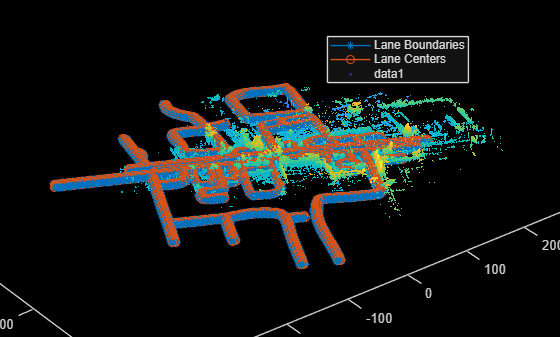
View the georeferenced point cloud and the overlaid RoadRunner HD Map. Observe that the xy-locations of the georeferenced point cloud align with the xy-locations of the road network in the RoadRunner HD Map. However, the OSM might not contain accurate elevation information, because of which the z-locations of the georeferenced point cloud might not align with the z-locations of the road network.
ax = plot(rrMap);
hold on
pcshow(georeferencedPointCloud,Parent=ax)
zoom(3)
title("Georeferenced Point Cloud Overlaid on OSM")
hold off
Summary
In this example, you learned how to register and stitch a sequence of point clouds obtained from a terrestrial lidar sensor to create a point cloud scene. You also learned how to georeference the stitched point cloud scene by using GPS sensor data.
You can use a georeferenced point cloud to add elevation information to maps such as an OpenStreetMap or RoadRunner HD Map. You can also extract static objects from a georeferenced point cloud to create a scene that spatially aligns these objects with a road network that has been reconstructed using OpenStreetMap. Additionally, you can use a georeferenced point cloud to add elevation to the scene data by using the addElevation function.
Helper Functions
function processedSensorData = helperRotatePointCloud(data,~)
    % Create a rigidtform3d object with rotation of 90 degrees in
    % anticlockwise direction.
    rotationAngle = [0 0 -90];
    translation = [0 0 0];
    tformLidarCoordinateSystem = rigidtform3d(rotationAngle,translation);

    % Create a new processedSensorData structure.
    processedSensorData = struct;
    processedSensorData.Timestamps = data.Timestamps;
    processedSensorData.PointClouds = {pctransform(data.PointClouds{1},tformLidarCoordinateSystem)};
    processedSensorData.Attributes = data.Attributes;
end
References
[1] Hesai and Scale. PandaSet. Accessed September 18, 2025. https://pandaset.org/. The PandaSet data set is provided under the CC-BY-4.0 license.
[2] You can download OpenStreetMap files from https://www.openstreetmap.org, which provides access to crowd-sourced map data all over the world. The data is licensed under the Open Data Commons Open Database License (ODbL), https://opendatacommons.org/licenses/odbl/.
See Also
Functions
roadrunnerStaticObjectInfo|lasFileReader(Lidar Toolbox) |readPointCloud(Lidar Toolbox) |addElevation