dsp.FarrowRateConverter
Polynomial sample rate converter with arbitrary conversion factor
Description
The dsp.FarrowRateConverter
System object™ implements a polynomial-fit sample rate conversion filter using a Farrow
structure. You can use this object to convert the sample rate of a signal up or down by an
arbitrary factor. This object supports fixed-point operations.
To convert the sample rate of a signal:
Create the
dsp.FarrowRateConverterobject and set its properties.Call the object with arguments, as if it were a function.
To learn more about how System objects work, see What Are System Objects?
Creation
Syntax
Description
frc = dsp.FarrowRateConverterfrc. For each channel of an input signal,
frc converts the input sample rate to the output sample
rate.
frc = dsp.FarrowRateConverter(PropertyName=Value)InputSampleRate to
45200.
Example: frc =
dsp.FarrowRateConverter(Specification="Coefficients",Coefficients=[1
2; 3 4]) returns a filter that converts from 44.1 kHz to
48 kHz using custom coefficients that implement a 2nd-order polynomial
filter.
frc = dsp.FarrowRateConverter(fsIn,fsOut,tol,np)frc, with InputSampleRate property set
to fsIn, OutputSampleRate property set
to fsOut, OutputRateTolerance
property set to tol, and PolynomialOrder property set
to np.
Properties
Unless otherwise indicated, properties are nontunable, which means you cannot change their
values after calling the object. Objects lock when you call them, and the
release function unlocks them.
If a property is tunable, you can change its value at any time.
For more information on changing property values, see System Design in MATLAB Using System Objects.
Filter Properties
Sample rate of the input signal, specified as a positive scalar in Hz. The input sample rate must be greater than the bandwidth of interest.
Data Types: single | double | int8 | int16 | int32 | int64 | uint8 | uint16 | uint32 | uint64
Sample rate of the output signal, specified as a positive scalar in Hz. The output sample rate can represent an upsample or downsample of the input signal.
Data Types: single | double | int8 | int16 | int32 | int64 | uint8 | uint16 | uint32 | uint64
Maximum tolerance for the output sample rate, specified as a positive scalar from 0 through 0.5, inclusive.
The actual output sample rate varies but is within the specified
range. For example, if OutputRateTolerance is
specified as 0.01, then the actual output sample
rate is in the range OutputSampleRate ±
1%. This flexibility often enables a simpler filter design.
Data Types: single | double | int8 | int16 | int32 | int64 | uint8 | uint16 | uint32 | uint64
Method for specifying filter coefficients for the interpolator filter, specified as one of the following:
"Polynomial order"— Use thePolynomialOrderproperty to specify the order of the Lagrange-interpolation-filter polynomial. The object calculates coefficients that meet the rate and tolerance properties."Coefficients"— Use theCoefficientsproperty to specify the polynomial coefficients directly.
Order of the Lagrange-interpolation-filter polynomial, specified as a positive integer less than or equal to 4. The object calculates coefficients that meet the rate and tolerance properties.
Dependencies
This property applies only when you set
Specification to "Polynomial
order".
Data Types: single | double | int8 | int16 | int32 | int64 | uint8 | uint16 | uint32 | uint64
Filter polynomial coefficients, specified as a real-valued M-by-M matrix, where M is the polynomial order.
The diagram shows the signal flow graph for a
dsp.FarrowRateConverter object with coefficients set to [1
2; 3 4].

Each branch of the FIR filter corresponds to a row of the coefficient matrix.
Dependencies
This property applies only when you set
Specification to
"Coefficients".
Data Types: single | double | int8 | int16 | int32 | int64 | uint8 | uint16 | uint32 | uint64
Fixed-Point Properties
Rounding method for fixed-point operations, specified as a character vector. For more information on the rounding methods see Rounding Modes.
Overflow action for fixed-point operations, specified as either
"Wrap" or "Saturate". For
more details on the overflow actions, see Overflow Handling.
Data type of the filter coefficients, specified as a signed numerictype (Fixed-Point Designer) object. The default data type is a signed, 16-bit
numerictype object. You must specify a
numerictype object without specific binary-point scaling. To
maximize precision, the object determines the fraction length of this data type based on
the coefficient values.
Data type of the fractional delay, specified as an unsigned
numerictype object. The default data type is an unsigned, 8-bit
numerictype object. You must specify a
numerictype object without specific binary-point scaling. To
maximize precision, the object determines the fraction length of this data type based on
the fractional delay values.
Data type of the multiplicand, specified as a signed numerictype
object. The default data type is a signed 16-bit numerictype object
with 13-bit fraction length. You must specify a numerictype object
that has a specific binary point scaling.
Data type of the output, specified as one of the following:
"Same word length as input"— Output word length and fraction length are the same as the input."Same as accumulator"— Output word length and fraction length are the same as the accumulator.numerictypeobject — Signed fixed-point output data type. If you do not specify a fraction length, the object computes the fraction length based on the input range. The object preserves the dynamic range of the input.
Usage
Syntax
Description
Input Arguments
Output Arguments
Object Functions
To use an object function, specify the
System object as the first input argument. For
example, to release system resources of a System object named obj, use
this syntax:
release(obj)
Examples
Note: The dsp.AudioFileWriter System object™ is not supported in MATLAB Online.
Create a dsp.FarrowRateConverter System object™ to convert an audio signal from 44.1 kHz to 96 kHz. Set the polynomial order for the filter.
FsIn = 44.1e3;
FsOut = 96e3;
LagrangeOrder = 2; % 1 = linear interpolation
frc = dsp.FarrowRateConverter(InputSampleRate=FsIn,...
                              OutputSampleRate=FsOut,...
                              PolynomialOrder=LagrangeOrder);
ar = dsp.AudioFileReader("guitar10min.ogg",SamplesPerFrame=14700);
aw = dsp.AudioFileWriter("guitar10min_96kHz.wav",SampleRate=FsOut);
Check the resulting interpolation and decimation factors.
[interp,decim] = getRateChangeFactors(frc)
interp =
320
decim =
147
Display the polynomial that the object uses to fit the input samples.
coeffs = getPolynomialCoefficients(frc)
coeffs = 3×3

    0.5000   -0.5000         0
   -1.0000         0    1.0000
    0.5000    0.5000         0
Convert 100 frames of the audio signal. Write the result to a file.
for n = 1:1:100
   x = ar();
   y = frc(x);
   aw(y);
end
Release the dsp.AudioFileWriter System object™ to complete creation of the output file.
release(aw)
release(ar)
Plot the input and output signals. The latency of the Farrow rate converter introduces a delay in the output signal.
tx = (0:length(x)-1)./FsIn;
ty = (0:length(y)-1)./FsOut;

figure

subplot(2,1,1)
plot(tx,x(:,1),".")
hold on
plot(ty,y(:,1),"--")
xlim([0 0.005])
xlabel("Time (s)")
legend("Input samples","Output samples","Location","best")
title("Channel 1")
subplot(2,1,2)
plot(tx,x(:,2),".")
hold on
plot(ty,y(:,2),"--")
xlim([0 0.005])
xlabel("Time (s)")
legend("Input samples","Output samples","Location","best")
title("Channel 2")
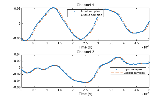
Use the outputDelay function to determine this delay value. To account for this delay, shift the output by this delay value.
[delay,~,~] = outputDelay(frc,Fc=0)
delay =
4.5351e-05
tx = (0:length(x)-1)./FsIn;
ty = (0:length(y)-1)./FsOut;

figure

subplot(2,1,1)
plot(tx,x(:,1),".")
hold on
plot(ty-delay,y(:,1),"--")
xlim([0 0.005])
xlabel("Time (s)")
legend("Input samples","Output samples","Location","best")
title("Channel 1")
subplot(2,1,2)
plot(tx,x(:,2),".")
hold on
plot(ty-delay,y(:,2),"--")
xlim([0 0.005])
xlabel("Time (s)")
legend("Input samples","Output samples","Location","best")
title("Channel 2")

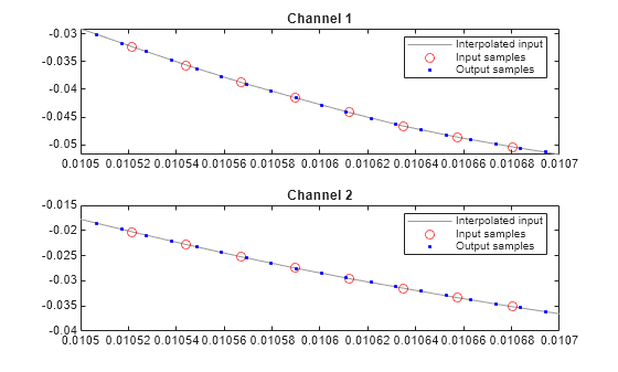
Zoom in to see the difference in sample rates.
figure
subplot(2,1,1)
plot(tx,x(:,1),Color=[0.6 0.6 0.6])
hold on
plot(tx,x(:,1),"ro")
plot(ty-delay,y(:,1),"b.")
xlim([0.0105 0.0107])
legend("Interpolated input","Input samples","Output samples")
title("Channel 1")
subplot(2,1,2)
plot(tx,x(:,2),Color=[0.6 0.6 0.6])
hold on
plot(tx,x(:,2),"ro")
plot(ty-delay,y(:,2),"b.")
xlim([0.0105 0.0107])
legend("Interpolated input","Input samples","Output samples")
title("Channel 2")
Create a dsp.FarrowRateConverter System object™ with 0% tolerance. The output rate is equal to the OutputSampleRate property. The input size must be a multiple of the decimation factor, M. In this case M is 320.
frc = dsp.FarrowRateConverter(InputSampleRate=96e3,...
    OutputSampleRate=44.1e3);
FsOut = getActualOutputRate(frc)
FsOut = 44100
[L,M] = getRateChangeFactors(frc)
L =
147
M =
320
Allow a 1% tolerance on the output rate and observe the difference in decimation factor.
frc.OutputRateTolerance = 0.01;
FsOut2 = getActualOutputRate(frc)
FsOut2 =
4.4308e+04
[L2,M2] = getRateChangeFactors(frc)
L2 =
6
M2 =
13
The decimation factor is now only 13. The lower the decimation factor, the more flexibility in input size. The output rate is within the range OutputSampleRate 1%.
Create a dsp.FarrowRateConverter System object™ with default properties. Compute and display the frequency response.
frc = dsp.FarrowRateConverter;
[h,f] = freqz(frc);
plot(f,20*log10(abs(h)))
ylabel("Filter Response")
xlabel("Frequency (rad/s)")

Create a dsp.FarrowRateConverter System object™ with default values. Determine its computational cost: the number of coefficients, number of states, multiplications per input sample, and additions per input sample.
frc = dsp.FarrowRateConverter;
cst = cost(frc)
cst = struct with fields:
                  NumCoefficients: 16
                        NumStates: 3
    MultiplicationsPerInputSample: 13.0612
          AdditionsPerInputSample: 11.9728
Repeat the computation, allowing for a 10% tolerance in the output sample rate.
frc.OutputRateTolerance = 0.1;
ctl = cost(frc)
ctl = struct with fields:
                  NumCoefficients: 16
                        NumStates: 3
    MultiplicationsPerInputSample: 12
          AdditionsPerInputSample: 11
More About
If the input is fixed point, it must be a signed integer or a signed fixed point value with a power-of-two slope and zero bias.
The diagram shows the data types that the dsp.FarrowRateConverter
object uses for fixed-point signals and floating-point signals. You can specify these data
types using the properties of the object, see Fixed-Point Properties. If the input is floating
point, all data types in filter are the same as the input data type,
single or double.

If the input is fixed point, the FIR filter defines internal data types using the
RoundingMode, OverflowMode, and
CoefficientsDataType properties. The accumulators and products within
the FIR filter use full precision data types. The object casts the output of the FIR filter
to MultiplicandDataType.
Algorithms
Farrow filters implement piecewise polynomial interpolation using Horner’s rule to compute samples from the polynomial. The polynomial coefficients used to fit the input samples correspond to the Lagrange interpolation coefficients.
Once a polynomial is fitted to the input data, the value of the polynomial can be calculated at any point. Therefore, a polynomial filter enables interpolation at arbitrary locations between input samples.
You can use a polynomial of any order to fit to the existing samples. However, since large-order polynomials frequently oscillate, polynomials of order 1, 2, 3, or 4 are used in practice.
The algorithm computes interpolated values at the desired locations by varying only the fractional delay µ. This value is the interval between the previous input sample and the current output sample. All filter coefficients remain constant.
The input samples are filtered using M + 1 FIR filters, where M is the polynomial order.
The outputs of these filters are multiplied by the fractional delay, µ.
The output is the sum of the multiplication results.
Here is the filter structure diagram of the Farrow filter with a polynomial order of 4.

References
[1] Hentschel, T., and G. Fettweis. "Continuous-Time Digital Filters for Sample-Rate Conversion in Reconfigurable Radio Terminals." Frequenz. Vol. 55, Number 5-6, 2001, pp. 185–188.
Extended Capabilities
Version History
Introduced in R2014bSee Also
Functions
getPolynomialCoefficients|getActualOutputRate|getRateChangeFactors|freqz|freqzmr|filterAnalyzer|info|cost|outputDelay|setInputSampleRate