hittime
Compute Markov chain hitting times
Syntax
Description
Examples
Consider this theoretical, right-stochastic transition matrix of a stochastic process.
Create the Markov chain that is characterized by the transition matrix P.
P = [1 0 0 0; 1/2 0 1/2 0; 0 0 0 1; 0 0 1/2 1/2];
mc = dtmc(P);
Plot a directed graph of the Markov chain. Visually identify the communicating class to which each state belongs by using node colors.
figure;
graphplot(mc,'ColorNodes',true);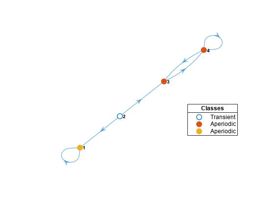
Compute the expected first hitting time for state 3, beginning from each state in the Markov chain.
ht = hittime(mc,3)
ht = 4×1

   Inf
   Inf
     0
     2
Because state 3 is unreachable from state 1, state 1 is a remote state with respect to state 3, with an expected first hitting time of Inf.
State 3 is reachable from state 2, but state 2 has a positive probability of transitioning to state 1, which is an absorbing state. Therefore, state 2 is a remote-reachable state with respect to state 3, with an expected first hitting time of Inf.
Because state 3 is the target, its expected first hitting time for itself is 0.
The expected first hitting time for state 3 starting from state 4 is 2 time steps.
Consider this theoretical, right-stochastic transition matrix of a stochastic process.
Create the Markov chain that is characterized by the transition matrix P.
P = [0   1/2 0   1/2
     2/3 0   1/3 0
     0   1/2 0   1/2
     1/3 0   2/3 0  ];
mc = dtmc(P);
Plot a digraph of the Markov chain mc. Display the transition probabilities.
graphplot(mc,'ColorEdges',true)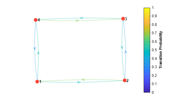
Compute the expected first hitting time for state 1, beginning from each state in the Markov chain.
ht = hittime(mc,1)
ht = 4×1

         0
    2.3333
    4.0000
    3.6667
Plot a digraph of the Markov chain. Specify node colors representing the expected first hitting times for state 1, beginning from each state in the Markov chain.
hittime(mc,1,'Graph',true);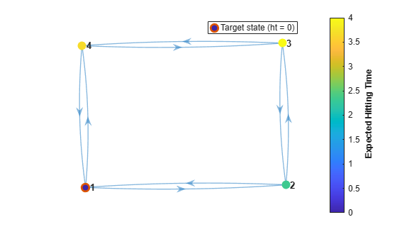
Plot another digraph. Include state 4 as a target state.
hittime(mc,[1 4],'Graph',true);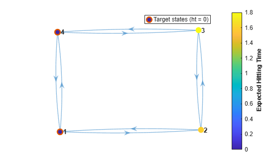
Create the Markov chain characterized by this transition matrix:
P = [1/2 0   1/2 0   0   0   0
     0   1/3 0   2/3 0   0   0
     1/4 0   3/4 0   0   0   0
     0   2/3 0   1/3 0   0   0
     1/4 1/8 1/8 1/8 1/4 1/8 0
     1/6 1/6 1/6 1/6 1/6 1/6 0
     1/2 0   0   0   0   0   1/2];
mc = dtmc(P);
Compute the expected first hitting times for state 1, beginning from each state in the Markov chain mc. Also, plot a digraph and specify node colors representing the expected first hitting times for state 1.
ht = hittime(mc,1,'Graph',true)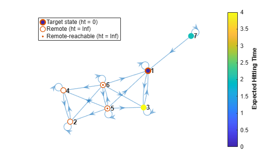
ht = 7×1

     0
   Inf
     4
   Inf
   Inf
   Inf
     2
States 2 and 4 form an absorbing class. Therefore, state 1 is unreachable from these states. The absorbing class is remote with respect to state 1, with an expected first hitting time of Inf.
State 1 is reachable from states 5 and 6, but the probability of transitioning into the absorbing class from states 5 and 6 is nonzero. Therefore, states 5 and 6 are remote-reachable with respect to state 1, with an expected first hitting time of Inf.
The expected first hitting time for state 1 beginning from state 7 is 2 time steps. The expected first hitting time for state 1 beginning from state 3 is 4 time steps.
Create an eight-state Markov chain from a randomly generated transition matrix with 50 infeasible transitions in random locations. An infeasible transition is a transition whose probability of occurring is zero. Assign arbitrary names to the states.
numStates = 8;
Zeros = 50;
stateNames = strcat(repmat("Regime ",1,8),string(1:8));
rng(1617676169) % For reproducibility
mc = mcmix(8,'Zeros',Zeros,'StateNames',stateNames);
Plot a digraph of the Markov chain mc. Specify node colors that identify transient and recurrent states and communicating classes.
figure;
graphplot(mc,'ColorNodes',true);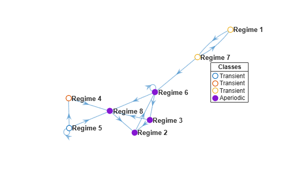
Find a recurrent class in the Markov chain mc by following this procedure:
Classify the states by passing
mctoclassify. Return the array of class membershipsClassStatesand the logical vector specifying whether the classes are recurrentClassRecurrence.Extract the recurrent classes from the array of classes by indexing into the array using the logical vector.
[~,ClassStates,IsClassRecurrent] = classify(mc);
recurrent = ClassStates{IsClassRecurrent}
recurrent = 1×4 string
"Regime 2" "Regime 3" "Regime 6" "Regime 8"
Compute the expected hitting time for the states of the recurrent class, beginning from each state in the Markov chain.
ht = hittime(mc,recurrent);
Extract and display the expected absorption times beginning from the transient states.
istransient = ~ismember(mc.StateNames,recurrent);
absorbtime = ht(istransient);
table(absorbtime,'RowNames',mc.StateNames(istransient))ans=4×1 table
absorbtime
__________
Regime 1 5.8929
Regime 4 1
Regime 5 1.7777
Regime 7 4.8929
Create a 50-state Markov chain from a random transition matrix in which most of the transitions are infeasible and randomly placed.
rng(1) % For reproducibility
mc = mcmix(50,'Zeros',2400);
Visualize the mixing time of the Markov chain by plotting a digraph and specifying node colors representing the expected first hitting times for state 1, beginning from each state.
hittime(mc,1,'Graph',true);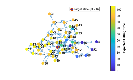
Visualize the mixing time of the Markov chain for state 5.
hittime(mc,5,'Graph',true);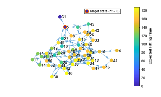
The expected commute time from state to state is the expected time required for a Markov chain to transition from state to state (the expected first hitting time ht), then back to state (ht). Formally, the expected commute time is
htht.
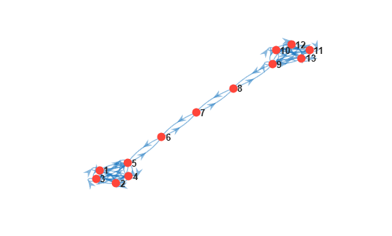
Create a "dumbbell" Markov chain containing 10 states in each "weight" and three states in the "bar."
Specify random transition probabilities between states within each weight.
If the Markov chain reaches the state in a weight that is closest to the bar, then specify a high probability of transitioning to the bar.
Specify uniform transitions between states in the bar.
rng(1); % For reproducibility
w = 5;                              % Dumbbell weights
DBar = [0 1 0; 1 0 1; 0 1 0];        % Dumbbell bar
DB = blkdiag(rand(w),DBar,rand(w));  % Transition matrix

% Connect dumbbell weights and bar
DB(w,w+1) = 1;
DB(w+1,w) = 1;
DB(w+3,w+4) = 1;
DB(w+4,w+3) = 1;

mc = dtmc(DB);
Plot a digraph of the Markov chain mc. Suppress node labels.
figure;
graphplot(mc);
Consider computing the expected commute time from state 1 to state 10.
Compute ht(1,10), the expected first hitting time for state 10 beginning from state 1.
ht = hittime(mc,10);
ht1to10 = ht(1);
Compute ht(10,1), the expected first hitting time for state 1 beginning from state 10.
ht = hittime(mc,1);
ht10to1 = ht(10);
Compute the expected commute time from state 1 to state 10.
C1to10 = ht1to10 + ht10to1
C1to10 =
236.6165
The expected commute time from state 1 to state 10 and back is 236.62 time steps.
Input Arguments
Output Arguments
More About
References
[1] Norris, J. R. Markov Chains. Cambridge, UK: Cambridge University Press, 1997.
Version History
Introduced in R2019b