VEC Model Monte Carlo Forecasts
This example shows how to generate Monte Carlo forecasts from a VEC(q) model. The example compares the generated forecasts to the minimum mean squared error (MMSE) forecasts and forecasts from the VAR(q+1) model equivalent of the VEC(q) model.
Suppose that a VEC(2) model with the H1 Johansen form appropriately describes the dynamics of a 3D multivariate time series composed of the annual short, medium, and long term bond rates from 1954 through 1994. Suppose that the series have a cointegration rank of 2.
Load and Preprocess Data
Load the Data_Canada data set. Extract the interest rate data, which occupy the third through last columns of the data.
load Data_Canada
Y = DataTable{:,3:end};
names = DataTable.Properties.VariableNames(3:end);
T = size(Y,1)
T = 41
numSeries = size(Y,2)
numSeries =
3
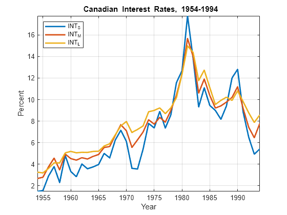
Plot the series in the same figure.
figure
plot(dates,Y,'LineWidth',2)
xlabel 'Year';
ylabel 'Percent';
legend(names,'Location','NW')
title '{\bf Canadian Interest Rates, 1954-1994}';
axis tight
grid on
Estimate VEC Model
Create a 3D VEC(2) model having a cointegration rank of 2.
numLags = 2;
r = 2;
Mdl = vecm(numSeries,r,numLags);
Estimate the VEC(2) model.
EstMdl = estimate(Mdl,Y);
By default, estimate applies the H1 Johansen form and uses the first q + 1 = 3 observations as presample data.
Generate Monte Carlo Forecasts
Generate Monte Carlo forecasts from the estimated VEC model over a 10-year horizon by using simulate. Provide the latest three rows of data to initialize the forecasts, and specify generating 1000 response paths.
numPaths = 1000;
horizon = 10;
Y0 = Y((end-2):end,:);

rng(1); % For reproducibility
YSimVEC = simulate(EstMdl,horizon,'NumPaths',numPaths,'Y0',Y0);
YSimVEC is a 10-by-3-by-1000 numeric array of simulated values of the response series. Rows correspond to periods in the forecast horizon, columns correspond to the series in Y, and pages correspond to simulated paths
Estimate the means of the forecasts for each period and time series over all paths. Construct 95% percentile forecast intervals for each period and time series.
YMCVEC   = mean(YSimVEC,3);
YMCVECCI = quantile(YSimVEC,[0.025,0.975],3);
YMCVEC is a 10-by-3 numeric matrix containing the Monte Carlo forecasts for each period (row) and time series (column). YMCVECCI is a 10-by-3-by-2 numeric array containing the 2.5% and 97.5% percentiles (pages) of the draws for each period (row) and time series (column).
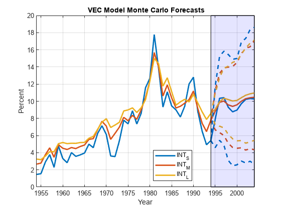
Plot the effective-sample observations, the mean forecasts, and the 95% percentile confidence intervals.
fDates = dates(end) + (0:horizon)';
figure;
h1 = plot([dates; fDates(2:end)],[Y; YMCVEC],'LineWidth',2);
h2 = gca;
hold on
h3 = plot(repmat(fDates,1,3),[Y(end,:,:); YMCVECCI(:,:,1)],'--',...
    'LineWidth',2);
h3(1).Color = h1(1).Color;
h3(2).Color = h1(2).Color;
h3(3).Color = h1(3).Color;
h4 = plot(repmat(fDates,1,3),[Y(end,:,:); YMCVECCI(:,:,2)],'--',...
    'LineWidth',2);
h4(1).Color = h1(1).Color;
h4(2).Color = h1(2).Color;
h4(3).Color = h1(3).Color;
patch([fDates(1) fDates(1) fDates(end) fDates(end)],...
    [h2.YLim(1) h2.YLim(2) h2.YLim(2) h2.YLim(1)],'b','FaceAlpha',0.1)
xlabel('Year')
ylabel('Percent')
title('{\bf VEC Model Monte Carlo Forecasts}')
axis tight
grid on
legend(h1,DataTable.Properties.VariableNames(3:end),'Location','Best');
Generate MMSE Forecasts
Estimate MMSE forecasts from the estimated VEC model over a 10-year horizon by using forecast. Provide the latest three rows of data to initialize the forecasts. Return the forecasts and respective, multivariate mean squared errors.
[YMMSE,YMMSEMSE] = forecast(EstMdl,horizon,Y0);
YMMSE is a 10-by-3 numeric matrix of MMSE forecasts. Rows correspond to periods in the forecast horizon and columns correspond to series in Y. YMMSEMSE is a 10-by-1 cell vector of 3-by-3 numeric matrices. The matrix in cell j is the estimated, multivariate MSE of the three forecasted values in period j. The diagonal values of the matrix are the forecast MSEs, and the off-diagonal values of the forecast covariances.
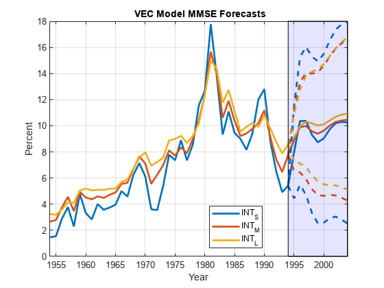
Estimate Wald-type 95% forecast intervals. Plot the MMSE forecasts and the forecast intervals.
YMMSECI = zeros(horizon,numSeries,2); % Preallocation
YMMSEMSE = cell2mat(cellfun(@(x)diag(x)',YMMSEMSE,'UniformOutput',false));
YMMSECI(:,:,1) = YMMSE - 1.96*sqrt(YMMSEMSE);
YMMSECI(:,:,2) = YMMSE + 1.96*sqrt(YMMSEMSE);

figure;
h1 = plot([dates; fDates(2:end)],[Y; YMMSE],'LineWidth',2);
h2 = gca;
hold on
h3 = plot(repmat(fDates,1,3),[Y(end,:,:); YMMSECI(:,:,1)],'--',...
    'LineWidth',2);
h3(1).Color = h1(1).Color;
h3(2).Color = h1(2).Color;
h3(3).Color = h1(3).Color;
h4 = plot(repmat(fDates,1,3),[Y(end,:,:); YMMSECI(:,:,2)],'--',...
    'LineWidth',2);
h4(1).Color = h1(1).Color;
h4(2).Color = h1(2).Color;
h4(3).Color = h1(3).Color;
patch([fDates(1) fDates(1) fDates(end) fDates(end)],...
    [h2.YLim(1) h2.YLim(2) h2.YLim(2) h2.YLim(1)],'b','FaceAlpha',0.1)
xlabel('Year')
ylabel('Percent')
title('{\bf VEC Model MMSE Forecasts}')
axis tight
grid on
legend(h1,DataTable.Properties.VariableNames(3:end),'Location','Best');
VAR(q + 1) Representation MMSE Forecasts
Represent the estimated VEC(2) as a VAR(3) model.
EstMdlVAR = varm(EstMdl)
EstMdlVAR =
  varm with properties:

     Description: "AR-Nonstationary 3-Dimensional VAR(3) Model"
     SeriesNames: "Y1"  "Y2"  "Y3"
       NumSeries: 3
               P: 3
        Constant: [-1.73631 -0.313676 0.0649337]'
              AR: {3×3 matrices} at lags [1 2 3]
           Trend: [3×1 vector of zeros]
            Beta: [3×0 matrix]
      Covariance: [3×3 matrix]
MdlVAR is a varm model object.
Estimate MMSE forecasts from the VAR model over a 10-year horizon by using forecast. Provide the latest three rows of data to initialize the forecasts. Return the forecasts and respective, multivariate mean squared errors.
[YMMSEVAR,YMMSEMSEVAR] = forecast(EstMdlVAR,horizon,Y0);
The dimensions of YMMSEVAR and YMMSEMSEVAR are the same as YMMSE and YMMSEMSE, respectively.
Estimate Wald-type 95% forecast intervals. Plot the MMSE forecasts and the forecast intervals.
YMMSEVARCI = zeros(horizon,numSeries,2);
YMMSEMSEVAR = cell2mat(cellfun(@(x)diag(x)',YMMSEMSEVAR,'UniformOutput',false));
YMMSEVARCI(:,:,1) = YMMSE - 1.96*sqrt(YMMSEMSEVAR);
YMMSEVARCI(:,:,2) = YMMSE + 1.96*sqrt(YMMSEMSEVAR);

figure;
h1 = plot([dates; fDates(2:end)],[Y; YMMSE],'LineWidth',2);
h2 = gca;
hold on
h3 = plot(repmat(fDates,1,3),[Y(end,:,:); YMMSEVARCI(:,:,1)],'--',...
    'LineWidth',2);
h3(1).Color = h1(1).Color;
h3(2).Color = h1(2).Color;
h3(3).Color = h1(3).Color;
h4 = plot(repmat(fDates,1,3),[Y(end,:,:); YMMSEVARCI(:,:,2)],'--',...
    'LineWidth',2);
h4(1).Color = h1(1).Color;
h4(2).Color = h1(2).Color;
h4(3).Color = h1(3).Color;
patch([fDates(1) fDates(1) fDates(end) fDates(end)],...
    [h2.YLim(1) h2.YLim(2) h2.YLim(2) h2.YLim(1)],'b','FaceAlpha',0.1)
xlabel('Year')
ylabel('Percent')
title('{\bf VAR Model MMSE Forecasts}')
axis tight
grid on
legend(h1,DataTable.Properties.VariableNames(3:end),'Location','Best');
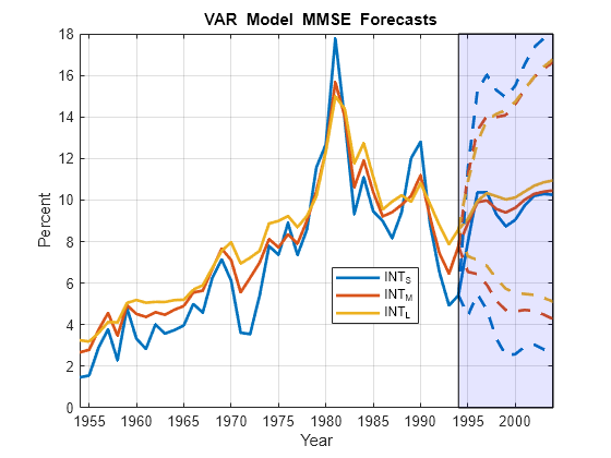
Confirm that the MMSE forecasts from the VEC and VAR models are the same.
(YMMSE - YMMSEVAR)'*(YMMSE - YMMSEVAR) > eps
ans = 3×3 logical array

   0   0   0
   0   0   0
   0   0   0
The MMSE forecasts between the models are identical.