twoRayChannel
Two-ray propagation channel
Description
The twoRayChannel
System object™ models a narrowband two-ray propagation channel. A two-ray propagation
channel is the simplest type of multipath channel. You can use a two-ray channel to
simulate propagation of signals in a homogeneous, isotropic medium with a single
reflecting boundary. This type of medium has two propagation paths: a line-of-sight
(direct) propagation path from one point to another and a ray path reflected from the
boundary. You can use the twoRayChannel object for short-range radar and
mobile communications applications where the signals propagate along straight paths and
the earth is assumed to be flat. You can also use this object for sonar and microphone
applications. For acoustic applications, you can choose the fields to be non-polarized
and adjust the propagation speed to be the speed of sound in air or water. You can use
twoRayChannel to model propagation from several points
simultaneously.
While the twoRayChannel object works for all frequencies, the
attenuation models for atmospheric gases and rain are valid for electromagnetic signals
in the frequency range 1–1000 GHz only. The attenuation model for fog and clouds is
valid for 10–1000 GHz. Outside these frequency ranges, the twoRayChannel
object uses the nearest valid value.
The twoRayChannel object applies range-dependent time delays to the
signals, and as well as gains or losses, phase shifts, and boundary reflection loss. The
twoRayChannel object also applies Doppler shift when either the
source or destination is moving.
Signals at the channel output can be kept separate or be
combined — controlled by the
CombinedRaysOutput property. In the
separate option, both fields arrive at the destination
separately and are not combined. For the combined option, the two
signals at the source propagate separately but are coherently summed at the destination
into a single quantity. This option is convenient when the difference between the sensor
or array gains in the directions of the two paths is not significant and need not be
taken into account.
Unlike the phased.FreeSpace
System object, the twoRayChannel
System object does not support two-way propagation.
To perform two-ray channel propagation:
Create the
twoRayChannelobject and set its properties.Call the object with arguments, as if it were a function.
To learn more about how System objects work, see What Are System Objects?
Creation
Description
channel = twoRayChannelchannel
System object.
channel = twoRayChannel(Name=Value)channel
System object with each specified property Name set to the
corresponding Value. You can specify additional pairs of
arguments in any order as
Name1=Value1,...,NameN=ValueN.
Properties
Usage
Description
prop_sig = channel(sig,origin_pos,dest_pos,origin_vel,dest_vel)prop_sig, when a narrowband
signal, sig, propagates through a two-ray channel from the
origin_pos position to the
dest_pos position. Either the
origin_pos or dest_pos arguments
can have multiple points but you cannot specify both as having multiple points.
The velocity of the signal origin is specified in
origin_vel and the velocity of the signal destination
is specified in dest_vel. The dimensions of
origin_vel and dest_vel must agree
with the dimensions of origin_pos and
dest_pos, respectively.
Electromagnetic fields propagated through a two-ray channel can be polarized
or nonpolarized. For, nonpolarized fields, such as an acoustic field, the
propagating signal field, sig, is a vector or matrix. When
the fields are polarized, sig is an array of structures.
Every structure element represents an electric field vector in Cartesian
form.
In the two-ray environment, there are two signal paths connecting every signal origin and destination pair. For N signal origins (or N signal destinations), there are 2N number of paths. The signals for each origin-destination pair do not have to be related. The signals along the two paths for any single source-destination pair can also differ due to phase or amplitude differences.
You can keep the two signals at the destination separate
or combined — controlled by the
CombinedRaysOutput property.
Combined means that the signals at the source propagate
separately along the two paths but are coherently summed at the destination into
a single quantity. To use the separate option, set
CombinedRaysOutput to false. To use
the combined option, set
CombinedRaysOutput to true. This
option is convenient when the difference between the sensor or array gains in
the directions of the two paths is not significant and need not be taken into
account.
Input Arguments
Output Arguments
Object Functions
To use an object function, specify the
System object as the first input argument. For
example, to release system resources of a System object named obj, use
this syntax:
release(obj)
Examples
This example illustrates the two-ray propagation of a signal, showing how the signals from the line-of-sight and reflected path arrive at the receiver at different times.
Create and Plot Propagating Signal
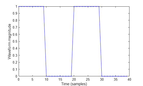
Create a nonpolarized electromagnetic field consisting of two rectangular waveform pulses at a carrier frequency of 100 MHz. Assume the pulse width is 10 ms and the sampling rate is 1 MHz. The bandwidth of the pulse is 0.1 MHz. Assume a 50% duty cycle in so that the pulse width is one-half the pulse repetition interval. Create a two-pulse wave train. Set the GroundReflectionCoefficient to 0.9 to model strong ground reflectivity. Propagate the field from a stationary source to a stationary receiver. The vertical separation of the source and receiver is approximately 10 km.
c = physconst('LightSpeed');
fs = 1e6;
pw = 10e-6;
pri = 2*pw;
PRF = 1/pri;
fc = 100e6;
lambda = c/fc;
waveform = phased.RectangularWaveform('SampleRate',fs,'PulseWidth',pw,...
    'PRF',PRF,'OutputFormat','Pulses','NumPulses',2);
wav = waveform();
n = size(wav,1);
figure;
plot((0:(n-1)),real(wav),'b.-');
xlabel('Time (samples)')
ylabel('Waveform magnitude')
Specify the Location of Source and Receiver
Place the source and receiver about 1000 meters apart horizontally and approximately 10 km apart vertically.
pos1 = [1000;0;10000];
pos2 = [0;100;100];
vel1 = [0;0;0];
vel2 = [0;0;0];
Compute the predicted signal delays in units of samples.
[rng,ang] = rangeangle(pos2,pos1,'two-ray');Create a Two-Ray Channel System Object™
Create a two-ray propagation channel System object™ and propagate the signal along both the line-of-sight and reflected ray paths.
channel = twoRayChannel('SampleRate',fs,...
    'GroundReflectionCoefficient',.9,'OperatingFrequency',fc,...
    'CombinedRaysOutput',false);
prop_signal = channel([wav,wav],pos1,pos2,vel1,vel2);
Plot the Propagated Signals
Plot the signal propagated along the line-of-sight.
Then, overlay a plot of the signal propagated along the reflected path.
Finally, overlay a plot of the coherent sum of the two signals.
n = size(prop_signal,1);
delay = 0:(n-1);
plot(delay,abs(prop_signal(:,1)),'g')
hold on
plot(delay,abs(prop_signal(:,2)),'r')
plot(delay,abs(prop_signal(:,1) + prop_signal(:,2)),'b')
hold off
legend('Line-of-sight','Reflected','Combined','Location','NorthWest')
xlabel('Delay (samples)')
ylabel('Signal Magnitude')
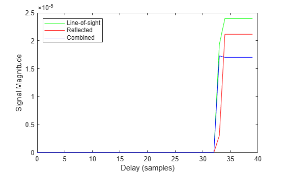
The plot shows that the delay of the reflected path signal agrees with the predicted delay. The magnitude of the coherently combined signal is less than either of the propagated signals indicating that there is some interference between the two signals.
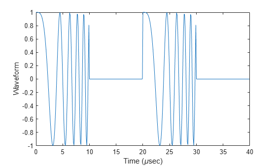
Create a polarized electromagnetic field consisting of linear FM waveform pulses. Propagate the field from a stationary source with a crossed-dipole antenna element to a stationary receiver approximately 10 km away. The transmitting antenna is 100 meters above the ground. The receiving antenna is 150 m above the ground. The receiving antenna is also a crossed-dipole. Plot the received signal.
Set Radar Waveform Parameters
Assume the pulse width is and the sampling rate is 10 MHz. The bandwidth of the pulse is 1 MHz. Assume a 50% duty cycle in which the pulse width is one-half the pulse repetition interval. Create a two-pulse wave train. Assume a carrier frequency of 100 MHz.
c = physconst('LightSpeed');
fs = 10e6;
pw = 10e-6;
pri = 2*pw;
PRF = 1/pri;
fc = 100e6;
bw = 1e6;
lambda = c/fc;
Set Up Required System Objects
Use a GroundRelativePermittivity of 10.
waveform = phased.LinearFMWaveform('SampleRate',fs,'PulseWidth',pw,...
    'PRF',PRF,'OutputFormat','Pulses','NumPulses',2,'SweepBandwidth',bw,...
    'SweepDirection','Up','Envelope','Rectangular','SweepInterval',...
    'Positive');
antenna = phased.CrossedDipoleAntennaElement(...
    'FrequencyRange',[50,200]*1e6);
radiator = phased.Radiator('Sensor',antenna,'OperatingFrequency',fc,...
    'Polarization','Combined');
channel = twoRayChannel('SampleRate',fs,...
    'OperatingFrequency',fc,'CombinedRaysOutput',false,...
    'EnablePolarization',true,'GroundRelativePermittivity',10);
collector = phased.Collector('Sensor',antenna,'OperatingFrequency',fc,...
    'Polarization','Combined');
Set Up Scene Geometry
Specify transmitter and receiver positions, velocities, and orientations. Place the source and receiver about 1000 m apart horizontally and approximately 50 m apart vertically.
posTx = [0;100;100];
posRx = [1000;0;150];
velTx = [0;0;0];
velRx = [0;0;0];
laxRx = rotz(180);
laxTx = rotx(1)*eye(3);
Create and Radiate Signals from Transmitter
Compute the transmission angles for the two rays traveling toward the receiver. These angles are defined with respect to the transmitter local coordinate system. The phased.Radiator System object™ uses these angles to apply separate antenna gains to the two signals.
[rng,angsTx] = rangeangle(posRx,posTx,laxTx,'two-ray');
wav = waveform();
Plot the transmitted Waveform
n = size(wav,1);
plot((0:(n-1))/fs*1000000,real(wav))
xlabel('Time ({\mu}sec)')
ylabel('Waveform')
sig = radiator(wav,angsTx,laxTx);
Propagate signals to receiver via two-ray channel
prop_sig = channel(sig,posTx,posRx,velTx,velRx);
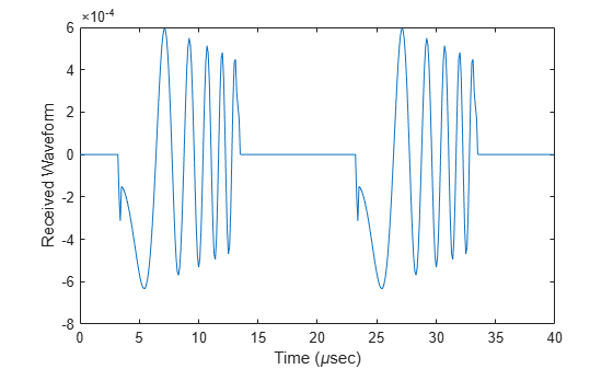
Receive Propagated Signal
Compute the reception angles for the two rays arriving at the receiver. These angles are defined with respect to the receiver local coordinate system. The phased.Collector System object™ uses these angles to apply separate antenna gains to the two signals.
[~,angsRx] = rangeangle(posTx,posRx,laxRx,'two-ray');Collect and combine received rays.
y = collector(prop_sig,angsRx,laxRx);
Plot received waveform
plot((0:(n-1))/fs*1000000,real(y))
xlabel('Time ({\mu}sec)')
ylabel('Received Waveform')
Propagate a signal in a two-ray channel environment from a radar at (0,0,10) meters to a target at (300,200,30) meters. Assume that the radar and target are stationary and that the transmitting antenna has a cosine pattern. Compare the combined signals from the two paths with the single signal resulting from free space propagation. Set the CombinedRaysOutput to true to produce a combined propagated signal.
Create a Rectangular Waveform
Set the sample rate to 2 MHz.
fs = 2e6;
waveform = phased.RectangularWaveform('SampleRate',fs);
wavfrm = waveform();
Create the Transmitting Antenna and Radiator
Set up a phased.Radiator System object™ to transmit from a cosine antenna
antenna = phased.CosineAntennaElement;
radiator = phased.Radiator('Sensor',antenna);
Specify Transmitter and Target Coordinates
posTx = [0;0;10];
posTgt = [300;200;30];
velTx = [0;0;0];
velTgt = [0;0;0];
Free Space Propagation
Compute the transmitting direction toward the target for the free-space model. Then, radiate the signal.
[~,angFS] = rangeangle(posTgt,posTx);
wavTx = radiator(wavfrm,angFS);
Propagate the signal to the target.
fschannel = phased.FreeSpace('SampleRate',waveform.SampleRate);
yfs = fschannel(wavTx,posTx,posTgt,velTx,velTgt);
release(radiator);
Two-Ray Propagation
Compute the two transmit angles toward the target for line-of-sight (LOS) path and reflected paths. Compute the transmitting directions toward the target for the two rays. Then, radiate the signals.
[~,angTwoRay] = rangeangle(posTgt,posTx,'two-ray');
wavTwoRay = radiator(wavfrm,angTwoRay);
Propagate the signals to the target.
channel = twoRayChannel('SampleRate',waveform.SampleRate,...
    'CombinedRaysOutput',true);
y2ray = channel(wavTwoRay,posTx,posTgt,velTx,velTgt);
Plot the Propagated Signals
Plot the combined signal against the free-space signal
plot(abs([y2ray yfs]))
legend('Two-ray','Free space')
xlabel('Samples')
ylabel('Signal Magnitude')

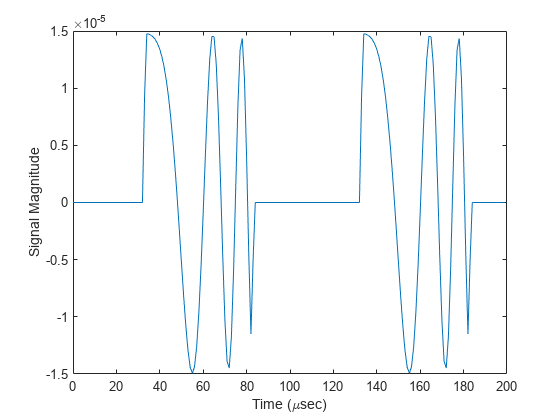
Propagate a linear FM signal in a two-ray channel. The signal propagates from a transmitter located at (1000,10,10) meters in the global coordinate system to a receiver at (10000,200,30) meters. Assume that the transmitter and the receiver are stationary and that they both have cosine antenna patterns. Plot the received signal.
Set up the radar scenario. First, create the required System objects.
waveform = phased.LinearFMWaveform('SampleRate',1000000,...
    'OutputFormat','Pulses','NumPulses',2);
fs = waveform.SampleRate;
antenna = phased.CosineAntennaElement;
radiator = phased.Radiator('Sensor',antenna);
collector = phased.Collector('Sensor',antenna);
channel = twoRayChannel('SampleRate',fs,...
    'CombinedRaysOutput',false,'GroundReflectionCoefficient',0.95);
Set up the scene geometry. Specify transmitter and receiver positions and velocities. The transmitter and receiver are stationary.
posTx = [1000;10;10];
posRx = [10000;200;30];
velTx = [0;0;0];
velRx = [0;0;0];
Specify the transmitting and receiving radar antenna orientations with respect to the global coordinates. The transmitting antenna points along the +x direction and the receiving antenna points near but not directly in the -x direction.
laxTx = eye(3);
laxRx = rotx(5)*rotz(170);
Compute the transmission angles which are the angles that the two rays traveling toward the receiver leave the transmitter. The phased.Radiator System object™ uses these angles to apply separate antenna gains to the two signals. Because the antenna gains depend on path direction, you must transmit and receive the two rays separately.
[~,angTx] = rangeangle(posRx,posTx,laxTx,'two-ray');Create and radiate signals from transmitter along the transmission directions.
wavfrm = waveform();
wavtrans = radiator(wavfrm,angTx);
Propagate signals to receiver via two-ray channel.
wavrcv = channel(wavtrans,posTx,posRx,velTx,velRx);
Collect signals at the receiver. Compute the angle at which the two rays traveling from the transmitter arrive at the receiver. The phased.Collector System object™ uses these angles to apply separate antenna gains to the two signals.
[~,angRcv] = rangeangle(posTx,posRx,laxRx,'two-ray');Collect and combine the two received rays.
yR = collector(wavrcv,angRcv);
Plot the received signals.
dt = 1/fs;
n = size(yR,1);
plot((0:(n-1))*dt*1000000,real(yR))
xlabel('Time ({\mu}sec)')
ylabel('Signal Magnitude')
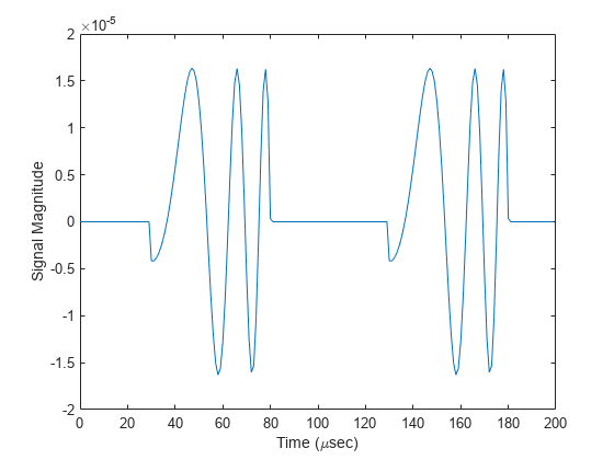
Propagate a 100 Mhz linear FM signal into a two-ray channel. Assume there is signal loss caused by atmospheric gases and rain. The signal propagates from a transmitter located at (0,0,0) meters in the global coordinate system to a receiver at (10000,200,30) meters. Assume that the transmitter and the receiver are stationary and that they both have cosine antenna patterns. Plot the received signal. Set the dry air pressure to 102.5 Pa and the rain rate to 5 mm/hr.
Set Up Radar Scenario
waveform = phased.LinearFMWaveform('SampleRate',1e6,...
    'OutputFormat','Pulses','NumPulses',2);
antenna = phased.CosineAntennaElement;
radiator = phased.Radiator('Sensor',antenna);
collector = phased.Collector('Sensor',antenna);
channel = twoRayChannel('SampleRate',waveform.SampleRate,...
    'CombinedRaysOutput',false,'GroundReflectionCoefficient',0.95,...
    'SpecifyAtmosphere',true,'Temperature',20,...
    'DryAirPressure',102.5,'RainRate',5.0);
Set up the scene geometry giving. the transmitter and receiver positions and velocities. The transmitter and receiver are stationary.
posTx = [0;0;0];
posRx = [10000;200;30];
velTx = [0;0;0];
velRx = [0;0;0];
Specify the transmitting and receiving radar antenna orientations with respect to the global coordinates. The transmitting antenna points along the +x-direction and the receiving antenna points close to the –x-direction.
laxTx = eye(3);
laxRx = rotx(5)*rotz(170);
Compute the transmission angles which are the angles that the two rays traveling toward the receiver leave the transmitter. The phased.Radiator System object™ uses these angles to apply separate antenna gains to the two signals. Because the antenna gains depend on path direction, you must transmit and receive the two rays separately.
[~,angTx] = rangeangle(posRx,posTx,laxTx,'two-ray');Create and Radiate Signals from Transmitter
Radiate the signals along the transmission directions.
wavfrm = waveform();
wavtrans = radiator(wavfrm,angTx);
Propagate signals to receiver via two-ray channel.
wavrcv = channel(wavtrans,posTx,posRx,velTx,velRx);
Collect Signal at Receiver
Compute the angle at which the two rays traveling from the transmitter arrive at the receiver. The phased.Collector System object™ uses these angles to apply separate antenna gains to the two signals.
[~,angRcv] = rangeangle(posTx,posRx,laxRx,'two-ray');Collect and combine the two received rays.
yR = collector(wavrcv,angRcv);
Plot Received Signal
dt = 1/waveform.SampleRate;
n = size(yR,1);
plot((0:(n-1))*dt*1000000,real(yR))
xlabel('Time ({\mu}sec)')
ylabel('Signal Magnitude')
More About
A two-ray propagation channel is the next step up in complexity from a free-space channel and is the simplest case of a multipath propagation environment. The free-space channel models a straight-line line-of-sight path from point 1 to point 2. In a two-ray channel, the medium is specified as a homogeneous, isotropic medium with a reflecting planar boundary. The boundary is always set at z = 0. There are at most two rays propagating from point 1 to point 2. The first ray path propagates along the same line-of-sight path as in the free-space channel. The line-of-sight path is often called the direct path. The second ray reflects off the boundary before propagating to point 2. According to the Law of Reflection , the angle of reflection equals the angle of incidence. In short-range simulations such as cellular communications systems and automotive radars, you can assume that the reflecting surface, the ground or ocean surface, is flat.
The twoRayChannel and widebandTwoRayChannel System objects model propagation time delay, phase
shift, Doppler shift, and loss effects for both paths. For the reflected path, loss effects
include reflection loss at the boundary.
The figure illustrates two propagation paths. From the source
position, ss, and the receiver
position, sr, you can compute
the arrival angles of both paths, θ′los and θ′rp.
The arrival angles are the elevation and azimuth angles of the arriving
radiation with respect to a local coordinate system. In this case,
the local coordinate system coincides with the global coordinate system.
You can also compute the transmitting angles, θlos and θrp.
In the global coordinates, the angle of reflection at the boundary
is the same as the angles θrp and θ′rp.
The reflection angle is important to know when you use angle-dependent
reflection-loss data. You can determine the reflection angle by using
the rangeangle function and
setting the reference axes to the global coordinate system. The total
path length for the line-of-sight path is shown in the figure by Rlos which
is equal to the geometric distance between source and receiver. The
total path length for the reflected path is Rrp=
R1 + R2. The
quantity L is the ground range between source and
receiver.

You can easily derive exact formulas for path lengths and angles in terms of the ground range and object heights in the global coordinate system.
References
[1] Saakian, A. Radio Wave Propagation Fundamentals. Norwood, MA: Artech House, 2011.
[2] Balanis, C. Advanced Engineering Electromagnetics. New York: Wiley & Sons, 1989.
[3] Rappaport, T. Wireless Communications: Principles and Practice, 2nd Ed New York: Prentice Hall, 2002.
[4] Radiocommunication Sector of the International Telecommunication Union. Recommendation ITU-R P.676-12: Attenuation by atmospheric gases. 2019.
[5] Radiocommunication Sector of the International Telecommunication Union. Recommendation ITU-R P.840-6: Attenuation due to clouds and fog. 2013.
[6] Radiocommunication Sector of the International Telecommunication Union. Recommendation ITU-R P.838-3: Specific attenuation model for rain for use in prediction methods. 2005.
Extended Capabilities
Version History
Introduced in R2021a