resubPredict

Classify training data using trained classifier

Syntax

label = resubPredict(Mdl)

[label,Score] = resubPredict(Mdl)

[label,Score] = resubPredict(Mdl,'IncludeInteractions',includeInteractions)

[label,Score,Cost] = resubPredict(Mdl)

Description

label = resubPredict(Mdl) returns a vector of predicted class labels (label) for the trained classification model Mdl using the predictor data stored in Mdl.X.

[label,Score] = resubPredict(Mdl) also returns classification scores.

[label,Score] = resubPredict(Mdl,'IncludeInteractions',includeInteractions) specifies whether to include interaction terms in computations. This syntax applies only to generalized additive models.

[label,Score,Cost] = resubPredict(Mdl) also returns the expected misclassification cost. This syntax applies only to k-nearest neighbor and naive Bayes models.

Examples

Label Training Sample Observations of Naive Bayes Classifier

Load the fisheriris data set. Create X as a numeric matrix that contains four measurements for 150 irises. Create Y as a cell array of character vectors that contains the corresponding iris species.

load fisheriris
X = meas;
Y = species;
rng('default') % For reproducibility

Train a naive Bayes classifier using the predictors X and class labels Y. A recommended practice is to specify the class names. fitcnb assumes that each predictor is conditionally and normally distributed.

Mdl = fitcnb(X,Y,'ClassNames',{'setosa','versicolor','virginica'})

Mdl = 
  ClassificationNaiveBayes
              ResponseName: 'Y'
     CategoricalPredictors: []
                ClassNames: {'setosa'  'versicolor'  'virginica'}
            ScoreTransform: 'none'
           NumObservations: 150
         DistributionNames: {'normal'  'normal'  'normal'  'normal'}
    DistributionParameters: {3×4 cell}


  Properties, Methods

Mdl is a trained ClassificationNaiveBayes classifier.

Predict the training sample labels.

label = resubPredict(Mdl);

Display the results for a random set of 10 observations.

idx = randsample(size(X,1),10);
table(Y(idx),label(idx),'VariableNames', ...
    {'True Label','Predicted Label'})

ans=10×2 table
      True Label      Predicted Label
    ______________    _______________

    {'virginica' }    {'virginica' } 
    {'setosa'    }    {'setosa'    } 
    {'virginica' }    {'virginica' } 
    {'versicolor'}    {'versicolor'} 
    {'virginica' }    {'virginica' } 
    {'versicolor'}    {'versicolor'} 
    {'virginica' }    {'virginica' } 
    {'setosa'    }    {'setosa'    } 
    {'virginica' }    {'virginica' } 
    {'setosa'    }    {'setosa'    } 

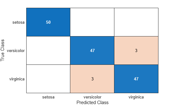
Create a confusion chart from the true labels Y and the predicted labels label.

cm = confusionchart(Y,label);

Estimate In-Sample Posterior Probabilities of SVM Classifier

Load the ionosphere data set. This data set has 34 predictors and 351 binary responses for radar returns, either bad ('b') or good ('g').

load ionosphere

Train a support vector machine (SVM) classifier. Standardize the data and specify that 'g' is the positive class.

SVMModel = fitcsvm(X,Y,'ClassNames',{'b','g'},'Standardize',true);

SVMModel is a ClassificationSVM classifier.

Fit the optimal score-to-posterior-probability transformation function.

rng(1); % For reproducibility
ScoreSVMModel = fitPosterior(SVMModel)

ScoreSVMModel = 
  ClassificationSVM
             ResponseName: 'Y'
    CategoricalPredictors: []
               ClassNames: {'b'  'g'}
           ScoreTransform: '@(S)sigmoid(S,-9.482430e-01,-1.217774e-01)'
          NumObservations: 351
                    Alpha: [90×1 double]
                     Bias: -0.1342
         KernelParameters: [1×1 struct]
                       Mu: [0.8917 0 0.6413 0.0444 0.6011 0.1159 0.5501 0.1194 0.5118 0.1813 0.4762 0.1550 0.4008 0.0934 0.3442 0.0711 0.3819 -0.0036 0.3594 -0.0240 0.3367 0.0083 0.3625 -0.0574 0.3961 -0.0712 0.5416 -0.0695 0.3784 … ] (1×34 double)
                    Sigma: [0.3112 0 0.4977 0.4414 0.5199 0.4608 0.4927 0.5207 0.5071 0.4839 0.5635 0.4948 0.6222 0.4949 0.6528 0.4584 0.6180 0.4968 0.6263 0.5191 0.6098 0.5182 0.6038 0.5275 0.5785 0.5085 0.5162 0.5500 0.5759 0.5080 … ] (1×34 double)
           BoxConstraints: [351×1 double]
          ConvergenceInfo: [1×1 struct]
          IsSupportVector: [351×1 logical]
                   Solver: 'SMO'


  Properties, Methods

Because the classes are inseparable, the score transformation function (ScoreSVMModel.ScoreTransform) is the sigmoid function.

Estimate scores and positive class posterior probabilities for the training data. Display the results for the first 10 observations.

[label,scores] = resubPredict(SVMModel);
[~,postProbs] = resubPredict(ScoreSVMModel);
table(Y(1:10),label(1:10),scores(1:10,2),postProbs(1:10,2),'VariableNames',...
    {'TrueLabel','PredictedLabel','Score','PosteriorProbability'})

ans=10×4 table
    TrueLabel    PredictedLabel     Score     PosteriorProbability
    _________    ______________    _______    ____________________

      {'g'}          {'g'}          1.4862           0.82216      
      {'b'}          {'b'}         -1.0003           0.30433      
      {'g'}          {'g'}          1.8685           0.86917      
      {'b'}          {'b'}         -2.6457          0.084171      
      {'g'}          {'g'}          1.2807           0.79186      
      {'b'}          {'b'}         -1.4616           0.22025      
      {'g'}          {'g'}          2.1674           0.89816      
      {'b'}          {'b'}         -5.7085           0.00501      
      {'g'}          {'g'}          2.4798           0.92224      
      {'b'}          {'b'}         -2.7812          0.074781      

Compare GAMs by Examining Logit of Posterior Probabilities

Estimate the logit of posterior probabilities (classification scores) for training data using a classification generalized additive model (GAM) that contains both linear and interaction terms for predictors. Specify whether to include interaction terms when computing the classification scores.

Load the ionosphere data set. This data set has 34 predictors and 351 binary responses for radar returns, either bad ('b') or good ('g').

load ionosphere

Train a GAM using the predictors X and class labels Y. A recommended practice is to specify the class names. Specify to include the 10 most important interaction terms.

Mdl = fitcgam(X,Y,'ClassNames',{'b','g'},'Interactions',10)

Mdl = 
  ClassificationGAM
             ResponseName: 'Y'
    CategoricalPredictors: []
               ClassNames: {'b'  'g'}
           ScoreTransform: 'logit'
                Intercept: 3.2565
             Interactions: [10×2 double]
          NumObservations: 351


  Properties, Methods

Mdl is a ClassificationGAM model object.

Predict the labels using both linear and interaction terms, and then using only linear terms. To exclude interaction terms, specify 'IncludeInteractions',false. Estimate the logit of posterior probabilities by specifying the ScoreTransform property as 'none'.

Mdl.ScoreTransform = 'none';
[labels,scores] = resubPredict(Mdl);
[labels_nointeraction,scores_nointeraction] = resubPredict(Mdl,'IncludeInteractions',false);

Create a table containing the true labels, predicted labels, and scores. Display the first eight rows of the table.

t = table(Y,labels,scores,labels_nointeraction,scores_nointeraction, ...
    'VariableNames',{'True Labels','Predicted Labels','Scores' ...
    'Predicted Labels Without Interactions','Scores Without Interactions'});
head(t)

    True Labels    Predicted Labels          Scores          Predicted Labels Without Interactions    Scores Without Interactions
    ___________    ________________    __________________    _____________________________________    ___________________________

       {'g'}            {'g'}          -51.628     51.628                    {'g'}                        -47.676     47.676     
       {'b'}            {'b'}           37.433    -37.433                    {'b'}                         36.435    -36.435     
       {'g'}            {'g'}          -62.061     62.061                    {'g'}                        -58.357     58.357     
       {'b'}            {'b'}           37.666    -37.666                    {'b'}                         36.297    -36.297     
       {'g'}            {'g'}          -47.361     47.361                    {'g'}                        -43.373     43.373     
       {'b'}            {'b'}           106.48    -106.48                    {'b'}                         102.43    -102.43     
       {'g'}            {'g'}          -62.665     62.665                    {'g'}                        -58.377     58.377     
       {'b'}            {'b'}           201.46    -201.46                    {'b'}                         197.84    -197.84     

The predicted labels for the training data X do not vary depending on the inclusion of interaction terms, but the estimated score values are different.

Estimate In-Sample Posterior Probabilities and Misclassification Costs of Naive Bayes Classifier

Estimate in-sample posterior probabilities and misclassification costs using a naive Bayes classifier.

Load the fisheriris data set. Create X as a numeric matrix that contains four measurements for 150 irises. Create Y as a cell array of character vectors that contains the corresponding iris species.

load fisheriris
X = meas;
Y = species;
rng('default') % For reproducibility

Train a naive Bayes classifier using the predictors X and class labels Y. A recommended practice is to specify the class names. fitcnb assumes that each predictor is conditionally and normally distributed.

Mdl = fitcnb(X,Y,'ClassNames',{'setosa','versicolor','virginica'});

Mdl is a trained ClassificationNaiveBayes classifier.

Estimate the posterior probabilities and expected misclassification costs for the training data.

[label,Posterior,MisclassCost] = resubPredict(Mdl);
Mdl.ClassNames

ans = 3×1 cell
    {'setosa'    }
    {'versicolor'}
    {'virginica' }

Display the results for 10 randomly selected observations.

idx = randsample(size(X,1),10);
table(Y(idx),label(idx),Posterior(idx,:),MisclassCost(idx,:),'VariableNames', ...
    {'TrueLabel','PredictedLabel','PosteriorProbability','MisclassificationCost'})

ans=10×4 table
      TrueLabel       PredictedLabel              PosteriorProbability                       MisclassificationCost         
    ______________    ______________    _________________________________________    ______________________________________

    {'virginica' }    {'virginica' }    6.2514e-269     1.1709e-09              1             1             1    1.1709e-09
    {'setosa'    }    {'setosa'    }              1     5.5339e-19      2.485e-25    5.5339e-19             1             1
    {'virginica' }    {'virginica' }    7.4191e-249     1.4481e-10              1             1             1    1.4481e-10
    {'versicolor'}    {'versicolor'}     3.4472e-62        0.99997      3.362e-05             1     3.362e-05       0.99997
    {'virginica' }    {'virginica' }    3.4268e-229      6.597e-09              1             1             1     6.597e-09
    {'versicolor'}    {'versicolor'}     6.0941e-77         0.9998     0.00019663             1    0.00019663        0.9998
    {'virginica' }    {'virginica' }    1.3467e-167       0.002187        0.99781             1       0.99781      0.002187
    {'setosa'    }    {'setosa'    }              1     1.5776e-15     5.7172e-24    1.5776e-15             1             1
    {'virginica' }    {'virginica' }    2.0116e-232     2.6206e-10              1             1             1    2.6206e-10
    {'setosa'    }    {'setosa'    }              1     1.8085e-17     1.9639e-24    1.8085e-17             1             1

The order of the columns of Posterior and MisclassCost corresponds to the order of the classes in Mdl.ClassNames.

Input Arguments

Mdl — Classification machine learning model

full classification model object

Classification machine learning model, specified as a full classification model object, as given in the following table of supported models.

Model	Classification Model Object
Generalized additive model	ClassificationGAM
k-nearest neighbor model	ClassificationKNN
Naive Bayes model	ClassificationNaiveBayes
Neural network model	ClassificationNeuralNetwork
Support vector machine for one-class and binary classification	ClassificationSVM

includeInteractions — Flag to include interaction terms

true | false

Flag to include interaction terms of the model, specified as true or false. This argument is valid only for a generalized additive model (GAM). That is, you can specify this argument only when Mdl is ClassificationGAM.

The default value is true if Mdl contains interaction terms. The value must be false if the model does not contain interaction terms.

Data Types: logical

Output Arguments

label — Predicted class labels

categorical array | character array | logical vector | numeric vector | cell array of character vectors

Predicted class labels, returned as a categorical or character array, logical or numeric vector, or cell array of character vectors.

label has the same data type as the observed class labels that trained Mdl, and its length is equal to the number of observations in Mdl.X. (The software treats string arrays as cell arrays of character vectors.)

Score — Class scores

numeric matrix

Class scores, returned as a numeric matrix. Score has rows equal to the number of observations in Mdl.X and columns equal to the number of distinct classes in the training data (size(Mdl.ClassNames,1)).

Cost — Expected misclassification costs

numeric matrix

Expected misclassification costs, returned as a numeric matrix. This output applies only to k-nearest neighbor and naive Bayes models. That is, resubPredict returns Cost only when Mdl is ClassificationKNN or ClassificationNaiveBayes.

Cost has rows equal to the number of observations in Mdl.X and columns equal to the number of distinct classes in the training data (size(Mdl.ClassNames,1)).

Cost(j,k) is the expected misclassification cost of the observation in row j of Mdl.X predicted into class k (in class Mdl.ClassNames(k)).

Algorithms

resubPredict computes predictions according to the corresponding predict function of the object (Mdl). For a model-specific description, see the predict function reference pages in the following table.

Model	Classification Model Object (Mdl)	predict Object Function
Generalized additive model	ClassificationGAM	predict
k-nearest neighbor model	ClassificationKNN	predict
Naive Bayes model	ClassificationNaiveBayes	predict
Neural network model	ClassificationNeuralNetwork	predict
Support vector machine for one-class and binary classification	ClassificationSVM	predict

Extended Capabilities

GPU Arrays

Accelerate code by running on a graphics processing unit (GPU) using Parallel Computing Toolbox™.

Usage notes and limitations:

• This function fully supports GPU arrays for a trained classification model specified as a ClassificationKNN, ClassificationNeuralNetwork, or ClassificationSVM object.

For more information, see Run MATLAB Functions on a GPU (Parallel Computing Toolbox).

Version History

Introduced in R2012a

R2024b: Specify GPU arrays for neural network models (requires Parallel Computing Toolbox)

resubPredict fully supports GPU arrays for ClassificationNeuralNetwork.

R2023b: Observations with missing predictor values are used in resubstitution and cross-validation computations

Starting in R2023b, the following classification model object functions use observations with missing predictor values as part of resubstitution ("resub") and cross-validation ("kfold") computations for classification edges, losses, margins, and predictions.

Model Type	Model Objects	Object Functions
Discriminant analysis classification model	ClassificationDiscriminant	resubEdge, resubLoss, resubMargin, resubPredict
	ClassificationPartitionedModel	kfoldEdge, kfoldLoss, kfoldMargin, kfoldPredict
Ensemble of discriminant analysis learners for classification	ClassificationEnsemble	resubEdge, resubLoss, resubMargin, resubPredict
	ClassificationPartitionedEnsemble	kfoldEdge, kfoldLoss, kfoldMargin, kfoldPredict
Gaussian kernel classification model	ClassificationPartitionedKernel	kfoldEdge, kfoldLoss, kfoldMargin, kfoldPredict
	ClassificationPartitionedKernelECOC	kfoldEdge, kfoldLoss, kfoldMargin, kfoldPredict
Linear classification model	ClassificationPartitionedLinear	kfoldEdge, kfoldLoss, kfoldMargin, kfoldPredict
	ClassificationPartitionedLinearECOC	kfoldEdge, kfoldLoss, kfoldMargin, kfoldPredict
Neural network classification model	ClassificationNeuralNetwork	resubEdge, resubLoss, resubMargin, resubPredict
	ClassificationPartitionedModel	kfoldEdge, kfoldLoss, kfoldMargin, kfoldPredict
Support vector machine (SVM) classification model	ClassificationSVM	resubEdge, resubLoss, resubMargin, resubPredict
	ClassificationPartitionedModel	kfoldEdge, kfoldLoss, kfoldMargin, kfoldPredict

In previous releases, the software omitted observations with missing predictor values from the resubstitution and cross-validation computations.