reset

Reset incremental k-means clustering model

Since R2025a

Syntax

Mdl = reset(Mdl)

Description

Mdl = reset(Mdl) returns the incrementalKMeans model Mdl with reset k-means clustering properties. The function resets these properties:

• IsWarm to false

• Centroids to NaN

• ClusterCounts to 0

• NumTrainingObservations to 0

• Metrics to NaN

• Mu and Sigma to []

reset preserves the NumPredictors, NumClusters, EstimationPeriod, and WarmupPeriod properties of Mdl. However, if WarmupPeriod is 0, the reset function resets WarmupPeriod to the default value of 1000.

Examples

Reset Incremental k-Means Clustering Model

Create an incremental model for k-means clustering with two clusters and a warm-up period of 100 observations.

Mdl = incrementalKMeans(numClusters=2,WarmupPeriod=100)

Mdl = 
  incrementalKMeans

         IsWarm: 0
        Metrics: [1×2 table]
    NumClusters: 2
      Centroids: [2×0 double]
       Distance: "sqeuclidean"


  Properties, Methods

Mdl is an incrementalKMeans model object. All its properties are read-only.

Load and Preprocess Data

Load the New York city housing data set.

load NYCHousing2015.mat

The data set includes 10 variables with information on the sales of properties in New York City in 2015. Keep only the gross square footage and sale price predictors, and records with a gross square footage above 100 square feet and a sales price above $1000.

data = NYCHousing2015(:,{'GROSSSQUAREFEET','SALEPRICE'});
data = data((data.GROSSSQUAREFEET > 100 & data.SALEPRICE > 1000),:);

Convert the tabular data into a matrix that contains the logarithm of both predictors.

 X = table2array(log10(data));

Fit Incremental Model

Fit the incremental model Mdl to the records using the fit function. To simulate a data stream, fit the model in chunks of 500 records at a time. At each iteration:

• Process 500 observations.

• Calculate the simplified silhouette performance window metric using the current model and the incoming chunk of records.

• Store the metric value in metricBeforeFit to see how it evolves during training.

• If the metric value is smaller than 0.5, call the reset function to reset the model.

• Overwrite the previous incremental model with a new one fitted to the incoming chunk of records.

• Calculate the simplified silhouette performance window metric using the new model. Store the value in metricAfterFit to see how it evolves during training.

• Store the cumulative number of fitted records in numFittedObs to see how it evolves during training.

• Store centroid1values and centroid2values (the predictor values of the two cluster centroids) to see how they evolve during training.

n = numel(data(:,1));
numObsPerChunk = 500;
nchunk = floor(n/numObsPerChunk);
metricBeforeFit = zeros(nchunk,1);
metricAfterFit  = zeros(nchunk,1);
numFittedObs = zeros(nchunk,1);
centroid1Values = zeros(nchunk,2);
centroid2Values = zeros(nchunk,2);
% Incremental fitting
for j = 1:nchunk
    ibegin = min(n,numObsPerChunk*(j-1) + 1);
    iend = min(n,numObsPerChunk*j);
    idx = ibegin:iend; 
    Mdl = updateMetrics(Mdl,X(idx,:));
    metricBeforeFit(j) = Mdl.Metrics.Window;
    if metricBeforeFit(j) < 0.5
        Mdl = reset(Mdl);
    end
    Mdl = fit(Mdl,X(idx,:));
    Mdl = updateMetrics(Mdl,X(idx,:));
    metricAfterFit(j) = Mdl.Metrics.Window;
    numFittedObs(j) = Mdl.NumTrainingObservations;
    centroid1Values(j,:) = Mdl.Centroids(1,:);
    centroid2Values(j,:) = Mdl.Centroids(2,:);
end

After the final iteration, call the assignClusters function to return the cluster index assignments for the records.

idx = assignClusters(Mdl,X);

Display a scatter plot of the two predictors. Color each point according to its cluster assignment. Plot the cluster centroid locations at the end of each iteration, and mark the values at the final iteration with filled pentagram symbols.

hold on
scatter(X(:,1),X(:,2),1,idx)
plot(centroid1Values(:,1),centroid1Values(:,2),'.-',color="cyan")
plot(centroid2Values(:,1),centroid2Values(:,2),'.-',color="r")
plot(centroid1Values(end,1),centroid1Values(end,2), ...
    Marker="pentagram",MarkerSize=15,MarkerFaceColor="cyan")
plot(centroid2Values(end,1),centroid2Values(end,2), ...
    Marker="pentagram",MarkerSize=15,MarkerFaceColor="red")
xlabel("log Gross Square Footage");
ylabel("log Sales Price in Dollars")
legend("","Centroid 1","Centroid 2","",Location="northwest")
hold off

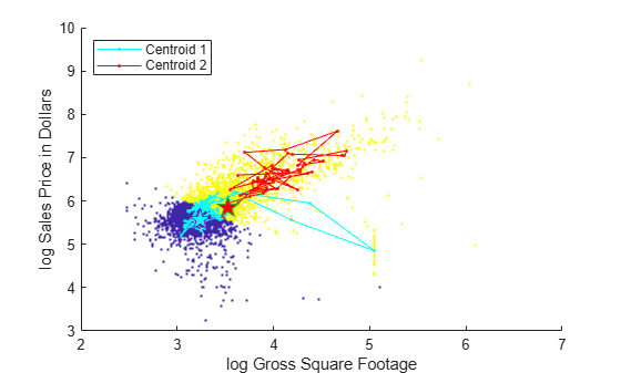
The plot shows that after the final iteration, the fitted cluster centroids are located near the overall center of the data distribution. However, at one iteration, the first fitted cluster centroid location deviates significantly from the center of the distribution.

To see where this deviation occurs, plot the performance metric values metricBeforeFit and metricAfterFit, and the cumulative number of fitted records at each iteration.

figure 
tiledlayout(2,1)
nexttile
plot([metricBeforeFit,metricAfterFit],'-o');
xlabel("Iteration")
ylabel("Performance Metric")
legend(["metricBeforeFit","metricAfterFit"],Location="southeast")
nexttile
plot(numFittedObs,'-o')
xlabel("Iteration")
ylabel("# of Fitted Observations")

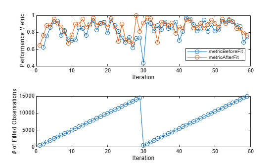
The top panel shows that the metricBeforeFit value drops significantly at the 30th iteration. Because this value is less than 0.5, the software calls the reset function, which resets the centroid positions, cluster counts, and cumulative number of fitted records in the incremental model. The software then fits the model and recalculates the performance metric. The resulting metricAfterFit value at the 30th iteration is greater than 0.8.

Input Arguments

Mdl — Incremental k-means clustering model

incrementalKMeans model object

Incremental k-means clustering model, specified as an incrementalKMeans model object. You can create Mdl by calling incrementalKMeans directly.

Version History

Introduced in R2025a