updateMetrics
Update performance metrics in incremental k-means clustering model given new data
Since R2025a
Description
returns a k-means clustering model Mdl
= updateMetrics(Mdl
,X
)Mdl
, which is the
input incrementalKMeans
model object Mdl
modified to
contain the model performance metrics on the incoming predictor data
X
.
When the input model is warm (Mdl.IsWarm
is true
),
updateMetrics
overwrites the previously computed metrics, stored in the
Metrics
property, with the new values. Otherwise,
updateMetrics
stores NaN
values in
Metrics
.
Examples
Create an incremental model for k-means clustering that has two clusters.
Mdl = incrementalKMeans(numClusters=2)
Mdl = incrementalKMeans IsWarm: 0 Metrics: [1×2 table] NumClusters: 2 Centroids: [2×0 double] Distance: "sqeuclidean" Properties, Methods
Mdl
is an incrementalKMeans
model object. All its properties are read-only.
Load and Preprocess Data
Load the New York city housing data set.
load NYCHousing2015.mat
The data set includes 10 variables with information on the sales of properties in New York City in 2015. Keep only the gross square footage and sale price predictors. Keep all records that have a gross square footage above 100 square feet and a sales price above $1000.
data = NYCHousing2015(:,{'GROSSSQUAREFEET','SALEPRICE'}); data = data((data.GROSSSQUAREFEET > 100 & data.SALEPRICE > 1000),:);
Convert the tabular data into a matrix that contains the logarithm of both predictors.
X = table2array(log10(data));
Randomly shuffle the order of the records.
rng(0,"twister"); % For reproducibility X = X(randperm(size(X,1)),:);
Fit and Plot Incremental Model
Fit the incremental model Mdl
to the data by using the fit
function. To simulate a data stream, fit the model in chunks of 500 records at a time. At each iteration:
Process 500 observations.
Overwrite the previous incremental model with a new one fitted to the incoming records.
Update the performance metrics for the model. The default metric for
Mdl
isSimplifiedSilhouette
.Store the cumulative and window metrics to see how they evolve during incremental learning.
Compute the cluster assignments of all records seen so far, according to the current model.
Plot all records seen so far, and color each record by its cluster assignment.
Plot the current centroid location of each cluster.
In this workflow, the updateMetrics
function provides information about the model's clustering performance after it is fit to the incoming data chunk. In other workflows, you might want to evaluate a clustering model's performance on unseen data. In such cases, you can call updateMetrics
prior to calling the incremental fit
function.
% Initialize plot properties hold on h1 = scatter(NaN,NaN,0.3); h2 = plot(NaN,NaN,Marker="o", ... MarkerFaceColor="k",MarkerEdgeColor="k"); h3 = plot(NaN,NaN,Marker="^", ... MarkerFaceColor="b",MarkerEdgeColor="b"); colormap(gca,"prism") pbaspect([1,1,1]) xlim([min(X(:,1)),max(X(:,1))]); ylim([min(X(:,2)),max(X(:,2))]); xlabel("log Gross Square Footage"); ylabel("log Sales Price in Dollars") % Incremental fitting and plotting n = numel(X(:,1)); numObsPerChunk = 500; nchunk = floor(n/numObsPerChunk); sil = array2table(zeros(nchunk,2),VariableNames=["Cumulative" "Window"]); for j = 1:nchunk ibegin = min(n,numObsPerChunk*(j-1) + 1); iend = min(n,numObsPerChunk*j); idx = ibegin:iend; Mdl = fit(Mdl,X(idx,:)); Mdl = updateMetrics(Mdl,X(idx,:)); sil{j,:} = Mdl.Metrics{'SimplifiedSilhouette',:}; indices = assignClusters(Mdl,X(1:iend,:)); title("Iteration " + num2str(j)) set(h1,XData=X(1:iend,1),YData=X(1:iend,2),CData=indices); set(h2,Marker="none") % Erase previous centroid markers set(h3,Marker="none") set(h2,XData=Mdl.Centroids(1,1),YData=Mdl.Centroids(1,2),Marker="o") set(h3,Xdata=Mdl.Centroids(2,1),YData=Mdl.Centroids(2,2),Marker="^") pause(0.5); end
Warning: Hardware-accelerated graphics is unavailable. Displaying fewer markers to preserve interactivity.
hold off
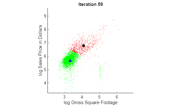
To view the animated figure, you can run the example, or open the animated gif below in your web browser.
At each iteration, the animated plot displays all the observations processed so far as small circles, and colors them according to the cluster assignments of the current model. The black circle indicates the centroid position of cluster 1, and the blue triangle indicates the centroid position of cluster 2.
Plot the window and cumulative metrics values at each iteration.
h4 = plot(sil.Variables); xlabel("Iteration") ylabel("Performance Metric") xline(Mdl.WarmupPeriod/numObsPerChunk,'g-.') legend(h4,sil.Properties.VariableNames,Location="southeast")
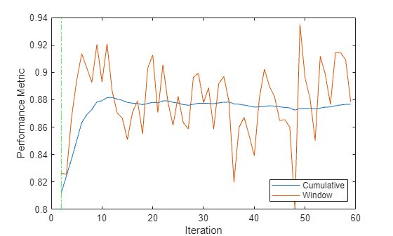
The updateMetrics
function calculates the performance metrics after the end of the warm-up period. The performance metrics rise rapidly from an initial value of 0.81
and approach a value of approximately 0.88
after 10 iterations.
Input Arguments
Incremental k-means clustering model, specified as an incrementalKMeans
model object. You can create Mdl
by
calling incrementalKMeans
directly.
Chunk of predictor data, specified as an
n-by-Mdl.NumPredictors
numeric matrix. The rows
of X
correspond to observations, and the columns correspond to
variables. The software ignores observations that contain at least one missing
value.
Note
updateMetrics
supports
only numeric input predictor data. If your input data includes categorical data, you
must prepare an encoded version of the categorical data. Use dummyvar
to convert each categorical variable to a numeric matrix of
dummy variables. Then, concatenate all dummy variable matrices and any other numeric
predictors. For more details, see Dummy Variables.
Data Types: single
| double
Output Arguments
Updated incremental k-means clustering model, returned as an
incrementalKMeans
model object.
If the input model Mdl
is not
warm (Mdl.IsWarm
is false
),
updateMetrics
does not compute performance metrics. As a result,
the Metrics
property of the output model Mdl
contains only NaN
values. If the input model is warm,
updateMetrics
computes the cumulative and window performance
metrics on the new data X
, and overwrites the corresponding
elements of Mdl.Metrics
. All other properties of the input model
carry over to the output model. For more details, see Performance Metrics.
More About
The updateMetrics
function tracks the model performance metrics in
Mdl.Metrics
from new data when the incremental model is warm
(Mdl.IsWarm
property). An incremental model becomes warm after
fit
fits the
incremental model to WarmupPeriod
observations, which is the
warm-up period. The default performance metric for an incrementalKMeans
model object is "SimplifiedSilhouette"
. For more details, see Simplified Silhouette.
If Mdl.EstimationPeriod
> 0, the software estimates
hyperparameters before fitting the model to data. Therefore, the software must process an
additional EstimationPeriod
observations before the model starts the
warm-up period.
The Metrics
property of the incremental model stores two forms of
each performance metric as variables (columns) of a table, Cumulative
and
Window
, with individual metrics in rows. When the incremental model is
warm, updateMetrics
updates the metrics at the following frequencies:
Cumulative
— The functions compute cumulative metrics since the start of model performance tracking. The functions update metrics every time you call the functions, and base the calculation on the entire supplied data set until a model reset.Window
— The functions compute metrics based on all observations within a window determined by theMetricsWindowSize
name-value argument.MetricsWindowSize
also determines the frequency at which the software updatesWindow
metrics. For example, ifMetricsWindowSize
is 20, the functions compute metrics based on the last 20 observations in the supplied data (X((end – 20 + 1):end,:)
andY((end – 20 + 1):end)
).Incremental functions that track performance metrics within a window use the following process:
Store
MetricsWindowSize
amount of values for each specified metric.Populate elements of the metrics values with the model performance based on batches of incoming observations.
When the window of observations is filled, overwrite
Mdl.Metrics.Window
with the average performance in the metrics window. If the window is overfilled when the function processes a batch of observations, the latest incomingMetricsWindowSize
observations are stored, and the earliest observations are removed from the window. For example, supposeMetricsWindowSize
is 20, the window contains 10 stored values from a previously processed batch, and 15 values are incoming. To compose the length 20 window, the functions use the measurements from the 15 incoming observations and the latest 5 measurements from the previous batch.
The software omits an observation with a NaN
cluster index when
computing the Cumulative
and Window
performance metric
values.
The simplified silhouette value si for the ith point is defined as
where ap,i is the distance of
the ith point to the centroid of its cluster p[1].
bp,i is the distance of the
ith point to the centroid of its closest neighboring cluster. If the
ith point is the only point in its cluster, then the simplified
silhouette value of the point is 1
.
The simplified silhouette values range from –1
to 1
.
A high value indicates that the point is well matched to its own cluster and poorly matched
to other clusters. If most points have a high simplified silhouette value, then the
clustering solution is appropriate. If many points have a low or negative simplified
silhouette value, then the clustering solution might have too many or too few clusters. You
can use simplified silhouette values as a clustering evaluation criterion with any distance
metric. By default, the performance metric values stored in the model object are the average
simplified silhouette values for all points passed to the updateMetrics
function.
References
[1] Vendramin, Lucas, Ricardo J.G.B. Campello, and Eduardo R. Hruschka. On the Comparison of Relative Clustering Validity Criteria. In Proceedings of the 2009 SIAM international conference on data mining, 733–744. Society for Industrial and Applied Mathematics, 2009.
Version History
Introduced in R2025a
MATLAB Command
You clicked a link that corresponds to this MATLAB command:
Run the command by entering it in the MATLAB Command Window. Web browsers do not support MATLAB commands.
Select a Web Site
Choose a web site to get translated content where available and see local events and offers. Based on your location, we recommend that you select: .
You can also select a web site from the following list
How to Get Best Site Performance
Select the China site (in Chinese or English) for best site performance. Other MathWorks country sites are not optimized for visits from your location.
Americas
- América Latina (Español)
- Canada (English)
- United States (English)
Europe
- Belgium (English)
- Denmark (English)
- Deutschland (Deutsch)
- España (Español)
- Finland (English)
- France (Français)
- Ireland (English)
- Italia (Italiano)
- Luxembourg (English)
- Netherlands (English)
- Norway (English)
- Österreich (Deutsch)
- Portugal (English)
- Sweden (English)
- Switzerland
- United Kingdom (English)