bagOfFeaturesDBoW

R2026b

Bag of visual words using DBoW2 library

Since R2024b

Description

Use the bagOfFeaturesDBoW object to create a bag of words (BoW) vocabulary to use for loop closure detection with vSLAM algorithms. This object uses the distributed bag of words DBoW2 library. This object supports oriented FAST and rotated BRIEF (ORB) and scale-invariant feature transform (SIFT) features.

Creation

Syntax

bag = bagOfFeaturesDBoW(imds)

bag = bagOfFeaturesDBoW(features)

bag = bagOfFeaturesDBoW(___,Name=Value)

bag = bagOfFeaturesDBoW(vocabularyFileName)

Description

bag = bagOfFeaturesDBoW() creates a bag of features with the default DBoW vocabulary file generated using ORB features. To use the default vocabulary file with SIFT features instead, specify the FeatureType name-value argument as "SIFT".

bag = bagOfFeaturesDBoW(imds) creates a bag of features from images specified by the datastore imds. The algorithm uses oriented fast and rotated brief (ORB) features by default to create the visual vocabulary. To use scale-invariant feature transform (SIFT) features instead, specify the FeatureType name-value argument as "SIFT".

bag = bagOfFeaturesDBoW(features) creates a bag of features from ORB or SIFT feature descriptors specified by features.

bag = bagOfFeaturesDBoW(___,Name=Value) sets properties by using one or more name-value arguments in addition to the previous syntax. For example, Normalization="L2" sets the normalization to L2.

bag = bagOfFeaturesDBoW(vocabularyFileName) loads an existing DBoW vocabulary file.

Input Arguments

imds — Images

ImageDatastore object

Images, specified as an ImageDatastore object.

features — ORB or SIFT feature descriptors

cell array of binaryFeatures | cell array of feature vectors

ORB or SIFT feature descriptors, specified as a cell array of binaryFeatures objects or feature vectors, respectively.

vocabularyFileName — DBoW vocabulary file

character string

DBoW vocabulary file, specified as a character string.

Name-Value Arguments

Specify optional pairs of arguments as Name1=Value1,...,NameN=ValueN, where Name is the argument name and Value is the corresponding value. Name-value arguments must appear after other arguments, but the order of the pairs does not matter.

FeatureType — Type of features used to construct DBoW vocabulary

"ORB" (default) | "SIFT"

Type of features used to construct the DBoW vocabulary, specified as "ORB" or "SIFT".

TreeProperties — Vocabulary tree properties

[5 10] (default) | 2-element vector

Vocabulary tree properties, specified as a 2-element vector of the form [depthLevel,branchingFactor]. depthLevel is the number of levels in the vocabulary tree, specified as an integer. branchingFactor is the factor to control the amount that the vocabulary can grow at successive levels in the tree, specified as an integer.

The capacity of a vocabulary tree to represent visual words is determined by the formula: branchingFactor x depthLevel. Commonly, the depthLevel ranges from 1 to 6, while the branchingFactor varies between 10 and 500. To identify the optimal values for these parameters, conducting empirical analysis is recommended.

Increasing the branching factor enlarges the vocabulary, potentially improving the accuracy of image similarity assessments. However, this adjustment also leads to an increase in the time required to encode images. Implementing a vocabulary tree with multiple levels can facilitate the creation of vocabularies comprising over 10,000 visual words. Although this multi-level approach streamlines the encoding process for images associated with large vocabularies, it necessitates a more extended setup phase.

Alternatively, for vocabularies containing only 100 to 1,000 visual words, employing a tree with a single level is advisable. This configuration simplifies the structure and accelerates the creation process, albeit for smaller vocabularies.

Normalization — Type of normalization applied to features

L1 (default) | L2

Type of normalization applied to the features, specified as L1 or L2. Normalization is the method by which to evaluate the similarity or dissimilarity between the feature descriptors for the bag of features.

• L1 — Calculates the sum of the absolute values of the vector elements.

• L2 — Calculates the square root of the sum of the squared values of the vector elements.

Properties

DepthLevel — Number of levels in the vocabulary tree

Read-only: integer

This property is read-only.

Number of levels in the vocabulary tree, returned as an integer. The Normalization property sets this value.

The TreeProperties name-value argument sets this property.

BranchingFactor — Number of branches of every node

Read-only: integer

This property is read-only.

Number of branches of every node in the vocabulary tree, returned as an integer. The Normalization property sets this value.

The TreeProperties name-value argument sets this property.

Normalization — Type of normalization applied to features

L1 (default) | L2

Type of normalization applied to the features, returned as an L1 or L2.

The Normalization name-value argument sets this property.

FeatureType — Type of features used to construct DBoW vocabulary

"ORB" (default) | "SIFT"

Type of features used to construct the DBoW vocabulary, returned as "ORB" or "SIFT".

The FeatureType name-value argument sets this property.

Object Functions

similarityMatrix

Compute self-similarity matrix for a set of image features based on bag of words representation

Examples

Create Bag of Features Using an Existing Vocabulary File

Create a bag of features object using an existing distributed bag of words (DBoW) vocabulary file.

bag = bagOfFeaturesDBoW("bagOfFeatures.bin.gz")

bag = 
  bagOfFeaturesDBoW with properties:

         DepthLevel: 5
    BranchingFactor: 10
      Normalization: 'L1'
        FeatureType: 'ORB'

Create Bag of Features Using Image Datastore

Create an image datastore for a set of images with stop signs.

folder=fullfile(toolboxdir("vision"),"visiondata","stopSignImages");
imds=imageDatastore(folder);

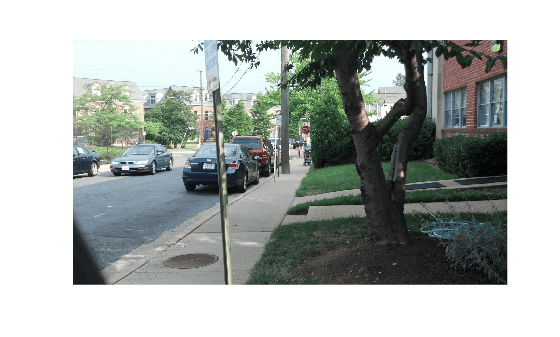
Visualize an image from the datastore.

imshow(preview(imds))

Create a bag of features vocabulary representation from the images in the datastore.

bag = bagOfFeaturesDBoW(imds)

bag = 
  bagOfFeaturesDBoW with properties:

         DepthLevel: 5
    BranchingFactor: 10
      Normalization: 'L1'
        FeatureType: 'ORB'

Create Bag of Features Using Image Features

Read an image.

I = imread("cameraman.tif");
imshow(I)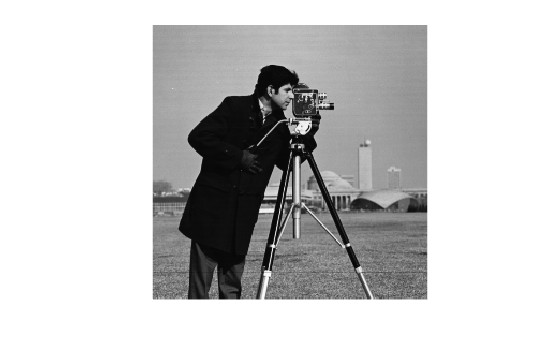

Detect ORB features in the image.

points = detectORBFeatures(I);
imshow(I)
hold on
plot(points,ShowScale=false)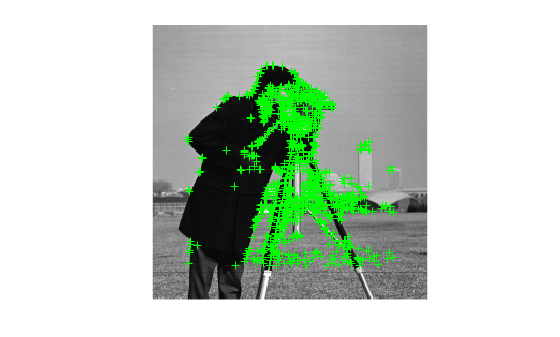

Extract ORB features from the detected points in the image. The extractFeatures function returns features and their corresponding locations. This code focuses on only the features for loop closure detection.

features = extractFeatures(I,points);

Create a bag of features using the extracted ORB features. Specify L2 normalization method to normalize image encodings in the bag.

bag = bagOfFeaturesDBoW({features},Normalization="L2")

bag = 
  bagOfFeaturesDBoW with properties:

         DepthLevel: 5
    BranchingFactor: 10
      Normalization: 'L2'
        FeatureType: 'ORB'

You can now apply this bag to tasks such as loop closure detection in visual SLAM workflows using the dbowLoopDetector object.

Compute Self-Similarity Matrix Using Bag of Features Created with SIFT Image Features

This example shows how to create a bag of words vocabulary using SIFT features extracted from images and compute self similarity matrix for all the images. It also shows how to use the computed similarity matrix to visualize images that are most similar to a given query image.

Load a set stop-sign images as an image datastore.

folder=fullfile(toolboxdir("vision"),"visiondata","stopSignImages");
imds=imageDatastore(folder);

Compute the scale-invariant feature transform (SIFT) features for all the images in the datastore.

siftFeatures = cell(numel(imds.Files),1);
for i = 1:numel(siftFeatures)
    img = rgb2gray(readimage(imds,i));
    siftFeatures{i} = extractFeatures(img,detectSIFTFeatures(img));
end

Create a bag of features object for the images using the bagofFeaturesDBoW object. To use SIFT image features while constructing the bag of features vocabulary, specify the FeatureType name-value argument as "SIFT".

bag = bagOfFeaturesDBoW(imds,FeatureType="SIFT");

Compute the similarity matrix for all the image features using the similarityMatrix object function. The function returns a sparse matrix that stores similarity scores for only the top visually similar images for each image feature, as specified by the StrongestResults name‑value argument. By default, each column has 10 nonzero similarity scores, and all other entries are zeros. Diagonal entries are 1 because each image is compared with itself, and all other similarity scores fall between 0 and 1, with higher values indicating stronger visual similarity.

You can adjust how many similar images are retained by specifying the StrongestResults name‑value argument.

simMatrix = similarityMatrix(bag,siftFeatures,StrongestResults=10)

simMatrix = 41×41

    1.0000    0.0675    0.0762    0.0600    0.0711         0         0    0.0605         0         0         0         0    0.0382         0         0         0         0         0         0         0         0    0.0594    0.0544         0         0    0.0534         0         0         0         0         0    0.0894    0.0856    0.0536    0.0915    0.0716         0    0.0570         0         0    0.0857
         0    1.0000    0.0891         0         0         0         0         0         0         0         0         0         0         0         0         0         0         0         0         0         0         0         0         0         0    0.0497         0         0         0         0    0.0598         0         0         0         0         0         0         0         0         0         0
         0    0.0891    1.0000         0         0         0         0         0         0         0         0         0         0         0         0         0         0         0         0         0         0         0         0         0         0    0.0488         0         0         0         0         0         0         0         0         0         0         0         0         0         0         0
         0         0         0    1.0000    0.0804         0         0         0         0         0         0         0         0         0         0         0         0         0         0         0         0    0.0612    0.0545         0         0         0         0         0         0         0         0         0         0    0.0549         0         0         0    0.0583         0         0         0
         0         0         0    0.0804    1.0000         0         0         0         0         0    0.0118         0    0.0363         0         0         0         0         0         0         0         0    0.0745    0.0604         0         0    0.0483         0         0         0         0         0         0         0    0.0617         0    0.0737    0.0427    0.0601    0.0286         0         0
    0.0885         0         0         0    0.0668    1.0000         0         0         0         0         0         0         0         0    0.1062    0.0947    0.1018    0.1001    0.1050         0    0.0882         0    0.0515         0         0         0         0         0         0         0         0    0.0986    0.0908         0         0         0         0    0.0537         0    0.1006    0.0906
         0         0         0         0         0         0    1.0000    0.1024    0.0791    0.0172    0.0203    0.0513         0         0         0         0         0         0         0    0.0401         0         0         0         0         0    0.0494    0.0238    0.0063         0    0.0689    0.0619         0         0         0         0         0         0         0         0         0         0
         0         0         0         0         0         0    0.1024    1.0000    0.1072    0.0106    0.0144    0.0355         0         0         0         0         0         0         0         0         0         0         0         0         0         0         0         0         0         0         0         0         0         0         0         0         0         0         0         0         0
         0         0         0         0         0         0    0.0791    0.1072    1.0000         0    0.0124    0.0429    0.0357         0         0         0         0         0         0         0         0         0         0         0         0    0.0514         0         0    0.0714    0.0709    0.0631         0         0         0         0         0         0         0         0         0         0
         0         0         0         0         0         0         0         0         0    1.0000    0.0889    0.0633         0         0         0         0         0         0         0         0         0         0         0         0         0         0         0    0.0075         0         0         0         0         0         0         0         0         0         0         0         0         0
         0         0         0         0         0         0         0         0         0    0.0889    1.0000    0.0760         0         0         0         0         0         0         0         0         0         0         0         0         0         0         0         0         0         0         0         0         0         0         0         0         0         0         0         0         0
         0         0         0         0         0         0         0         0         0    0.0633    0.0760    1.0000         0    0.0260         0         0         0         0         0         0         0         0         0         0         0         0         0    0.0073         0         0         0         0         0         0         0         0         0         0         0         0         0
         0         0         0         0         0         0         0         0         0         0         0         0    1.0000    0.0698         0         0         0         0         0         0         0         0         0         0         0         0         0         0         0         0         0         0         0         0         0         0    0.0558         0    0.0350         0         0
         0         0         0         0         0         0         0         0         0    0.0119         0         0    0.0698    1.0000         0         0         0         0         0         0         0         0         0         0         0         0         0         0         0         0         0         0         0         0         0         0    0.0478         0    0.0566         0         0
         0    0.0699    0.0789         0         0    0.1062    0.0699    0.0674    0.0813         0         0         0         0         0    1.0000    0.1187    0.1276    0.1160    0.1314    0.0385    0.0947         0         0    0.0904    0.0675         0    0.0238         0    0.0781    0.0815    0.0640    0.0969    0.0935         0    0.1016         0         0         0         0    0.1275    0.0966
      ⋮

Retrieve the indices of the images most similar to a selected query image. In this example, you extract the nonzero similarity entries for the 15th image, sort them in descending order of similarity score, and return the corresponding image indices.

queryImageIdx = 15;
idx = find(simMatrix(:,queryImageIdx));
[~,order] = sort(simMatrix(idx,queryImageIdx),"descend");
sortedIdx = idx(order)'

sortedIdx = 1×10

    15    19    17    40    16    18     6    35    32    41

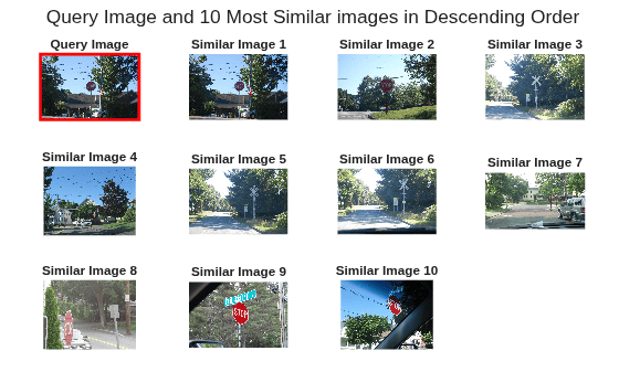
Visualize the query image and its 10 most similar images in the order of decreasing similarity scores. This helps you qualitatively inspect how well the similarity matrix captures visual similarity among the image features.

figure
tl = tiledlayout(3,4,TileSpacing="compact",Padding="compact");
title(tl,"Query Image and 10 Most Similar images in Descending Order")
nexttile
ax = gca;
imshow(readimage(imds,queryImageIdx))
hold on
rectangle(Position=[ax.XLim(1) ax.YLim(1) diff(ax.XLim) diff(ax.YLim)],Edgecolor="r",LineWidth=2)
title("Query Image")

for k = 1:numel(sortedIdx)
nexttile
    imshow(readimage(imds,sortedIdx(k)))
    title(sprintf("Similar Image %d", k))
end

References

[1] Galvez-López, D., and J. D. Tardos. “Bags of Binary Words for Fast Place Recognition in Image Sequences.” IEEE Transactions on Robotics, vol. 28, no. 5, Oct. 2012, pp. 1188–97. DOI.org (Crossref), https://doi.org/10.1109/TRO.2012.2197158.

Version History

Introduced in R2024b

R2026b: Support for Computing Similarity Matrix and Using SIFT Features to Create Visual Vocabulary

Starting in R2026b, you can:

• Create the bag of words vocabulary using SIFT features by specifying the FeatureType argument as "SIFT".

• Compute self-similarity matrix for a set of image features using the similarityMatrix object function, which represents visual similarity scores among all the images in the data set.