Results for
Cody often hides subtle hints in example outputs — like data shape, rounding, or format. Matching those exactly saves you a lot of debugging time.
The Cody Contest 2025 is underway, and it includes a super creative problem group which many of us have found fascinating. The central theme of the problems, expertly curated by @Matt Tearle, humorously revolves around the whims of the capricious dictator Lord Ned, as he goes out of his way to complicate the lives of his subjects and visitors alike. We cannot judge whether or not there's any truth to the rumors behind all the inside jokes, but it's obvious that the team had a lot of fun creating these; and we had even more fun solving them.
Today I want to showcase a way of graphically solving and visualizing one of those problems which I found very elegant, The Bridges of Nedsburg.
To briefly reiterate the problem, the number of islands and the arrangement of bridges of the city of Nedsburg are constantly changing. Lord Ned has decided to take advantage of this by charging visitors with an increasingly expensive n-bridge pass which allows them to cross up to n bridges in one journey. Given the Connectivity Matrix C, we are tasked with calculating the minimum n needed so that there is a path from every island to every other island in n steps or fewer.
Matt kindly provided us with some useful bit of math in the description detailing how to calculate the way to get from one island to another in an number of m steps. However, he has also hidden an alternative path to the solution in plain sight, in one of the graphs he provided. This involves the extremely useful and versatile class digraph, representing directed graphs, which have directional edges connecting the nodes. Here's some further great documentation and other cool resources on the topic for those who are interested in learning more about it:
Let's start using this class to explore a graphical solution to Lord Ned's conundrum. We will use the unit tests included in the problem to visualize the solution. We can retrieve the connectivity matrix for each case using the following function:
function C = getConnectivityMatrix(unit_test)
% Number of islands and bridge arrangement
switch unit_test
case 1
m = 3; idx = [3;4;8];
case 2
m = 3; idx = [3;4;7;8];
case 3
m = 4; idx = [2;7;8;10;13];
case 4
m = 4; idx = [4;5;7;8;9;14];
case 5
m = 5; idx = [5;8;11;12;14;18;22;23];
case 6
m = 5; idx = [2;5;8;14;20;21;24];
case 7
m = 6; idx = [3;4;7;11;18;23;24;26;30;32];
case 8
m = 6; idx = [3;11;12;13;18;19;28;32];
case 9
m = 7; idx = [3;4;6;8;13;14;20;21;23;31;36;47];
case 10
m = 7; idx = [4;11;13;14;19;22;23;26;28;30;34;35;37;38;45];
case 11
m = 8; idx = [2;4;5;6;8;12;13;17;27;39;44;48;54;58;60;62];
case 12
m = 8; idx = [3;9;12;20;24;29;30;31;33;44;48;50;53;54;58];
case 13
m = 9; idx = [8;9;10;14;15;22;25;26;29;33;36;42;44;47;48;50;53;54;55;67;80];
case 14
m = 9; idx = [8;10;22;32;37;40;43;45;47;53;56;57;62;64;69;70;73;77;79];
case 15
m = 10; idx = [2;5;8;13;16;20;24;27;28;36;43;49;53;62;71;75;77;83;86;87;95];
case 16
m = 10; idx = [4;9;14;21;22;35;37;38;44;47;50;51;53;55;59;61;63;66;69;76;77;84;85;86;90;97];
end
C = zeros(m);
C(idx) = 1;
end
The case in the example refers to unit test case 2.
unit_test = 2;
C = getConnectivityMatrix(unit_test);
disp(C)
D = digraph(C);
figure
p = plot(D,'LineWidth',1.5,'ArrowSize',10);
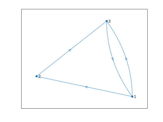
This is the same as the graph provided in the example. Another very useful method of digraph is shortestpath. This allows us to calculate the path and distance from one single node to another. For example:
% Path and distance from node 1 to node 2
[path12,dist12] = shortestpath(D,1,2);
fprintf('The shortest path from island %d to island %d is: %s. The minimum number of steps is: n = %d\n', 1, 2, join(string(path12), ' -> '),dist12)
% Path and distance from node 2 to node 1
[path21,dist21] = shortestpath(D,2,1);
fprintf('The shortest path from island %d to island %d is: %s. The minimum number of steps is: n = %d\n', 2, 1, join(string(path21), ' -> '),dist21)
figure
p = plot(D,'LineWidth',1.5,'ArrowSize',10);
highlight(p,path12,'EdgeColor','r','NodeColor','r','LineWidth',2)
highlight(p,path21,'EdgeColor',[0 0.8 0],'LineWidth',2)

But that's not all! digraph can also provide us with a matrix of the distances d, i.e. the steps needed to travel from island i to island j, where i and j are the rows and columns of d respectively. This is accomplished by using its distances method. The distance matrix can be visualized as:
d = distances(D);
figure
% Using pcolor w/ appending matrix workaround for convenience
pcolor([d,d(:,end);d(end,:),d(end,end)])
% Alternatively you can use imagesc(d), but you'll have to recreate the grid manually
axis square
set(gca,'YDir','reverse','XTick',[],'YTick',[])
[X,Y] = meshgrid(1:height(d));
text(X(:)+0.5,Y(:)+0.5,string(d(:)),'FontSize',11)
colormap(interp1(linspace(0,1,4), [1 1 1; 0.7 0.9 1; 0.6 0.7 1; 1 0.3 0.3], linspace(0,1,8)))
clim([-0.5 7+0.5])
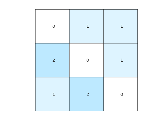
This confirms what we saw before, i.e. you need 1 step to go from island 1 to island 2, but 2 steps for vice versa. It also confirms that the minimum number of steps n that you need to buy the pass for is 2 (which also occurs for traveling from island 3 to island 2). As it's not the point of the post to give the full solution to the problem but rather present the graphical way of visualizing it I will not include the code of how to calculate this, but I'm sure that by now it's reduced to a trivial problem which you have already figured out how to solve.
That being said, now that we have the distance matrix, let's continue with the visualizations. First, let's plot the corresponding paths for each of these combinations:
figure
tiledlayout(size(C,1),size(C,2),'TileSpacing','tight','Padding','tight');
for i = 1:size(C,1)
for j = 1:size(C,2)
nexttile
p = plot(D,'ArrowSize',10);
highlight(p,shortestpath(D,i,j),'EdgeColor','r','NodeColor','r','LineWidth',2)
lims = axis;
text(lims(1)+diff(lims(1:2))*0.05,lims(3)+diff(lims(3:4))*0.9,sprintf('n = %d',d(i,j)))
end
end

This allows us to go from the distance matrix to visualizing the paths and number of steps for each corresponding case. Things are rather simple for this 3-island example case, but evil Lord Ned is just getting started. Let's now try to solve the problem for all provided unit test cases:
% Cell array of connectivity matrices
C = arrayfun(@getConnectivityMatrix,1:16,'UniformOutput',false);
% Cell array of corresponding digraph objects
D = cellfun(@digraph,C,'UniformOutput',false);
% Cell array of corresponding distance matrices
d = cellfun(@distances,D,'UniformOutput',false);
% id of solutions: Provided as is to avoid handing out the code to the full solution
id = [2, 2, 9, 3, 4, 6, 16, 4, 44, 43, 33, 34, 7, 18, 39, 2];
First, let's plot the distance matrix for each case:
figure
tiledlayout('flow','TileSpacing','compact','Padding','compact');
% Vary this to plot different combinations of cases
plot_cases = 1:numel(C);
for i = plot_cases
nexttile
pcolor([d{i},d{i}(:,end);d{i}(end,:),d{i}(end,end)])
axis square
set(gca,'YDir','reverse','XTick',[],'YTick',[])
title(sprintf('Case %d',i),'FontWeight','normal','FontSize',8)
end
c = colorbar('Ticks',0:7,'TickLength',0,'Limits',[-0.5 7+0.5],'FontSize',8);
c.Layout.Tile = 'East';
c.Label.String = 'Number of Steps';
c.Label.FontSize = 8;
colormap(interp1(linspace(0,1,4), [1 1 1; 0.7 0.9 1; 0.6 0.7 1; 1 0.3 0.3], linspace(0,1,8)))
clim(findobj(gcf,'type','axes'),[-0.5 7+0.5])
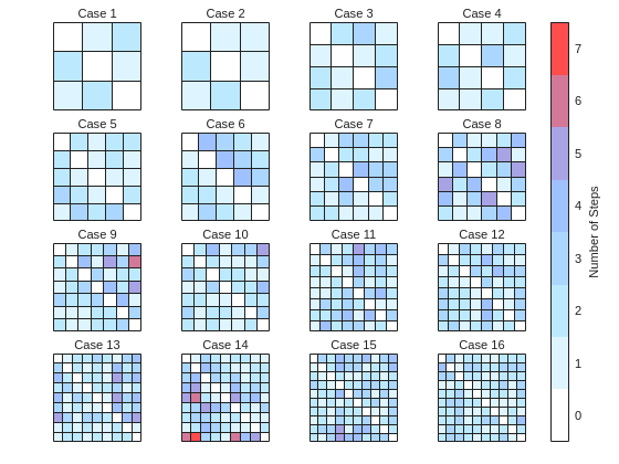
We immediately notice some inconsistencies, perhaps to be expected of the eccentric and cunning dictator. Things are pretty simple for the configurations with a small number of islands, but the minimum number of steps n can increase sharply and disproportionally to the additional number of islands. Cases 8 and 9 specifically have a particularly large n (relative to their grid dimensions), and case 14 has the largest n, almost double that of case 16 despite the fact that the latter has one extra island.
To visualize how this is possible, let's plot the path corresponding to the largest n for each case (though note that there might be multiple possible paths for each case):
figure
tiledlayout('flow','TileSpacing','tight','Padding','tight');
for i = plot_cases
nexttile
% Changing the layout to circular so we can better visualize the paths
p = plot(D{i},'ArrowSize',10,'Layout','Circle');
% Alternatively we could use the XData and YData properties if the positions of the islands were provided
axis([-1.5 1.5 -1.5 1.75])
[row,col] = ind2sub(size(d{i}),id(i));
highlight(p,shortestpath(D{i},row,col),'EdgeColor','r','NodeColor','r','LineWidth',2)
lims = axis;
text(lims(1)+diff(lims(1:2))*0.05,lims(3)+diff(lims(3:4))*0.9,sprintf('n = %d',d{i}(row,col)))
end
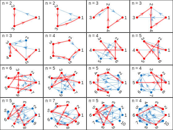
And busted! Unraveled! Exposed! Lord Ned has clearly been taking advantages of the tectonic forces by instructing his corrupt civil engineer lackeys to design the bridges to purposely force the visitors to go around in circles in order to drain them of their precious savings. In particular, for cases 8 and 9, he would have them go through every single island just to get from one island to another, whereas for case 14 they would have to visit 8 of the 9 islands just to get to their destination. If that's not diabolical then I don't know what is!
Ned jokes aside, I hope you enjoyed this contest just as much as I did, and that you found this article useful. I look forward to seeing more creative problems and solutions in the future.

It’s exciting to dive into a new dataset full of unfamiliar variables but it can also be overwhelming if you’re not sure where to start. Recently, I discovered some new interactive features in MATLAB live scripts that make it much easier to get an overview of your data. With just a few clicks, you can display sparklines and summary statistics using table variables, sort and filter variables, and even have MATLAB generate the corresponding code for reproducibility.
The Graphics and App Building blog published an article that walks through these features showing how to explore, clean, and analyze data—all without writing any code.
If you’re interested in streamlining your exploratory data analysis or want to see what’s new in live scripts, you might find it helpful:
If you’ve tried these features or have your own tips for quick data exploration in MATLAB, I’d love to hear your thoughts!
Pure Matlab
82%
Simulink
18%
11 votes
isequal() is your best friend for Cody! It compares arrays perfectly without rounding errors — much safer than == for matrix outputs.
When Cody hides test cases, test your function with random small inputs first. If it works for many edge cases, it will almost always pass the grader.
I am Prof Ansar Interested in coding challenge taker inmatlab
What a fantastic start to Cody Contest 2025! In just 2 days, over 300 players joined the fun, and we already have our first contest group finishers. A big shoutout to the first finisher from each team:
- Team Creative Coders: @Mehdi Dehghan
- Team Cool Coders: @Pawel
- Team Relentless Coders: @David Hill
- 🏆 First finisher overall: Mehdi Dehghan
Other group finishers: @Bin Jiang (Relentless), @Mazhar (Creative), @Vasilis Bellos (Creative), @Stefan Abendroth (Creative), @Armando Longobardi (Cool), @Cephas (Cool)
Kudos to all group finishers! 🎉
Reminder to finishers: The goal of Cody Contest is learning together. Share hints (not full solutions) to help your teammates complete the problem group. The winning team will be the one with the most group finishers — teamwork matters!
To all players: Don’t be shy about asking for help! When you do, show your work — include your code, error messages, and any details needed for others to reproduce your results.
Keep solving, keep sharing, and most importantly — have fun!
I realized that using vectorized logic instead of nested loops makes Cody problems run much faster and cleaner. Functions like any(), all(), and logical indexing can replace multiple for-loops easily !
Hi cool guys,
I hope you are coding so cool!
FYI, in Problem 61065. Convert Hexavigesimal to Decimal in Cody Contest 2025 there's a small issue with the text:
[ ... For example, the text ‘aloha’ would correspond to a vector of values [0 11 14 7 0], thus representing the base-26 value 202982 = 11*263 + 14*262 + 7*26 ...]
The bold section should be:
202982 = 11*26^3 + 14*26^2 + 7*26
The main round of Cody Contest 2025 kicks off today! Whether you’re a beginner or a seasoned solver, now’s your time to shine.
Here’s how to join the fun:
- Pick your team — choose one that matches your coding personality.
- Solve Cody problems — gain points and climb the leaderboard.
- Finish the Contest Problem Group — help your team win and unlock chances for weekly prizes by finishing the Cody Contest 2025 problem group.
- Share Tips & Tricks — post your insights to win a coveted MathWorks Yeti Bottle.
- Bonus Round — 2 players from each team will be invited to a fun live code-along event!
- Watch Party – join the big watch event to see how top players tackle Cody problems
Contest Timeline:
- Main Round: Nov 10 – Dec 7, 2025
- Bonus Round: Dec 8 – Dec 19, 2025
Big prizes await — MathWorks swag, Amazon gift cards, and shiny virtual badges!
We look forward to seeing you in the contest — learn, compete, and have fun!
Jorge Bernal-AlvizJorge Bernal-Alviz shared the following code that requires R2025a or later:
Test()

function Test()
duration = 10;
numFrames = 800;
frameInterval = duration / numFrames;
w = 400;
t = 0;
i_vals = 1:10000;
x_vals = i_vals;
y_vals = i_vals / 235;
r = linspace(0, 1, 300)';
g = linspace(0, 0.1, 300)';
b = linspace(1, 0, 300)';
r = r * 0.8 + 0.1;
g = g * 0.6 + 0.1;
b = b * 0.9 + 0.1;
customColormap = [r, g, b];
figure('Position', [100, 100, w, w], 'Color', [0, 0, 0]);
axis equal;
axis off;
xlim([0, w]);
ylim([0, w]);
hold on;
colormap default;
colormap(customColormap);
plothandle = scatter([], [], 1, 'filled', 'MarkerFaceAlpha', 0.12);
for i = 1:numFrames
t = t + pi/240;
k = (4 + 3 * sin(y_vals * 2 - t)) .* cos(x_vals / 29);
e = y_vals / 8 - 13;
d = sqrt(k.^2 + e.^2);
c = d - t;
q = 3 * sin(2 * k) + 0.3 ./ (k + 1e-10) + ...
sin(y_vals / 25) .* k .* (9 + 4 * sin(9 * e - 3 * d + 2 * t));
points_x = q + 30 * cos(c) + 200;
points_y = q .* sin(c) + 39 * d - 220;
points_y = w - points_y;
CData = (1 + sin(0.1 * (d - t))) / 3;
CData = max(0, min(1, CData));
set(plothandle, 'XData', points_x, 'YData', points_y, 'CData', CData);
brightness = 0.5 + 0.3 * sin(t * 0.2);
set(plothandle, 'MarkerFaceAlpha', brightness);
drawnow;
pause(frameInterval);
end
end
Hey Creative Coders! 😎
Let’s get to know each other. Drop a quick intro below and meet your teammates! This is your chance to meet teammates, find coding buddies, and build connections that make the contest more fun and rewarding!
You can share:
- Your name or nickname
- Where you’re from
- Your favorite coding topic or language
- What you’re most excited about in the contest
Let’s make Team Creative Coders an awesome community—jump in and say hi! 🚀
Hey Cool Coders! 😎
Let’s get to know each other. Drop a quick intro below and meet your teammates! This is your chance to meet teammates, find coding buddies, and build connections that make the contest more fun and rewarding!
You can share:
- Your name or nickname
- Where you’re from
- Your favorite coding topic or language
- What you’re most excited about in the contest
Let’s make Team Cool Coders an awesome community—jump in and say hi! 🚀
Welcome to the Cody Contest 2025 and the Creative Coders team channel! 🎉
You think outside the box. Where others see limitations, you see opportunities for innovation. This is your space to connect with like-minded coders, share insights, and help your team win. To make sure everyone has a great experience, please keep these tips in mind:
- Follow the Community Guidelines: Take a moment to review our community standards. Posts that don’t follow these guidelines may be flagged by moderators or community members.
- Ask Questions About Cody Problems: When asking for help, show your work! Include your code, error messages, and any details needed to reproduce your results. This helps others provide useful, targeted answers.
- Share Tips & Tricks: Knowledge sharing is key to success. When posting tips or solutions, explain how and why your approach works so others can learn your problem-solving methods.
- Provide Feedback: We value your feedback! Use this channel to report issues or share creative ideas to make the contest even better.
Have fun and enjoy the challenge! We hope you’ll learn new MATLAB skills, make great connections, and win amazing prizes! 🚀
Welcome to the Cody Contest 2025 and the Cool Coders team channel! 🎉
You stay calm under pressure. No panic, no chaos—just smooth problem-solving. This is your space to connect with like-minded coders, share insights, and help your team win. To make sure everyone has a great experience, please keep these tips in mind:
- Follow the Community Guidelines: Take a moment to review our community standards. Posts that don’t follow these guidelines may be flagged by moderators or community members.
- Ask Questions About Cody Problems: When asking for help, show your work! Include your code, error messages, and any details needed to reproduce your results. This helps others provide useful, targeted answers.
- Share Tips & Tricks: Knowledge sharing is key to success. When posting tips or solutions, explain how and why your approach works so others can learn your problem-solving methods.
- Provide Feedback: We value your feedback! Use this channel to report issues or share creative ideas to make the contest even better.
Have fun and enjoy the challenge! We hope you’ll learn new MATLAB skills, make great connections, and win amazing prizes! 🚀
I just learned you can access MATLAB Online from the following shortcut in your web browser: https://matlab.new
Thanks @Yann Debray
From his recent blog post: pip & uv in MATLAB Online » Artificial Intelligence - MATLAB & Simulink
Inspired by @xingxingcui's post about old MATLAB versions and @유장's post about an old Easter egg, I thought it might be fun to share some MATLAB-Old-Timer Stories™.
Back in the early 90s, MATLAB had been ported to MacOS, but there were some interesting wrinkles. One that kept me earning my money as a computer lab tutor was that MATLAB required file names to follow Windows standards - no spaces or other special characters. But on a Mac, nothing stopped you from naming your script "hello world - 123.m". The problem came when you tried to run it. MATLAB was essentially doing an eval on the script name, assuming the file name would follow Windows (and MATLAB) naming rules.
So now imagine a lab full of students taking a university course. As is common in many universities, the course was given a numeric code. For whatever historical reason, my school at that time was also using numeric codes for the departments. Despite being told the rules for naming scripts, many students would default to something like "26.165 - 1.1" for problem one on HW1 for the intro applied math course 26.165.
No matter what they did in their script, when they ran it, MATLAB would just say "ans = 25.0650".
Nothing brings you more MATLAB-god credibility as a student tutor than walking over to someone's computer, taking one look at their output, saying "rename your file", and walking away like a boss.
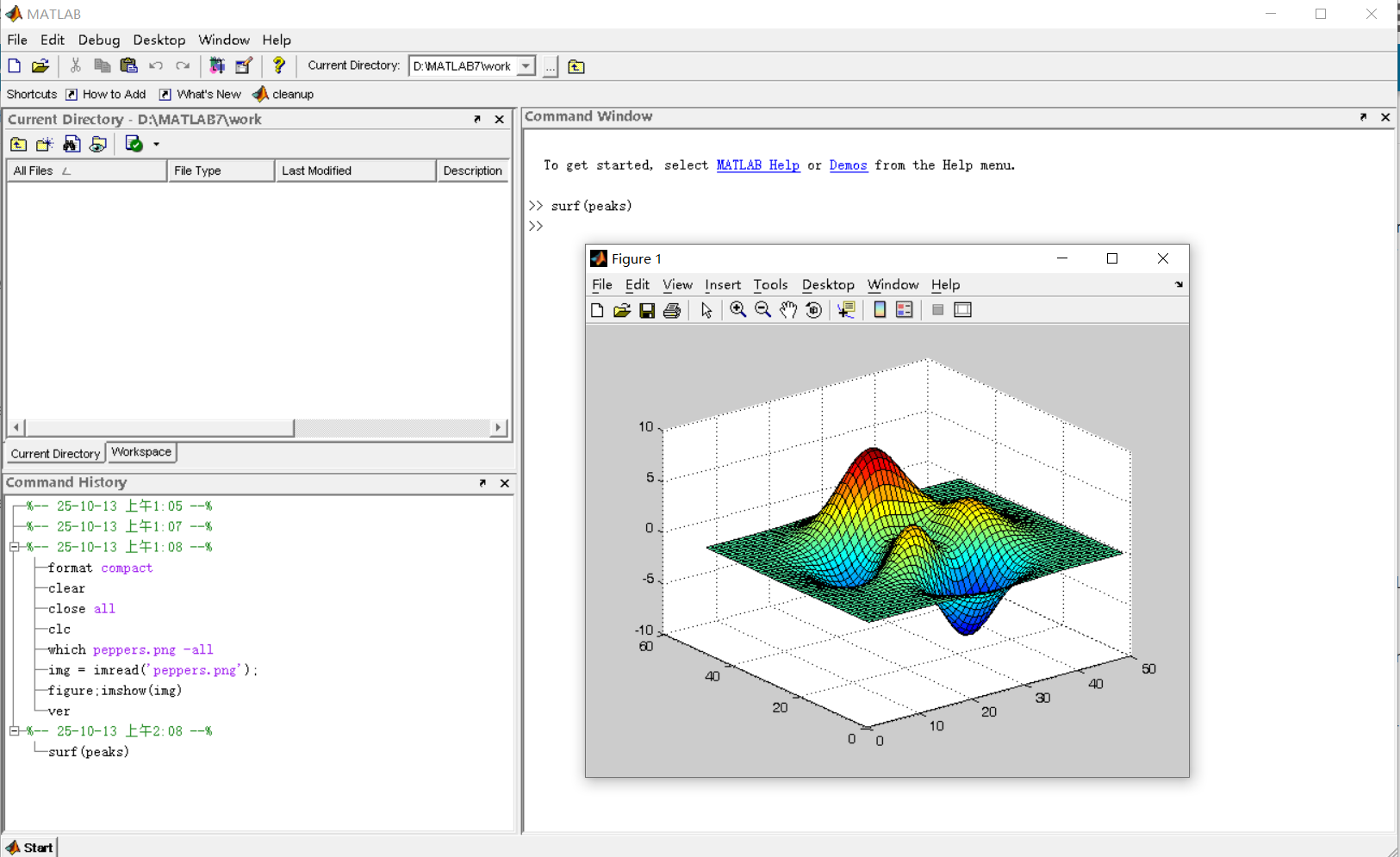
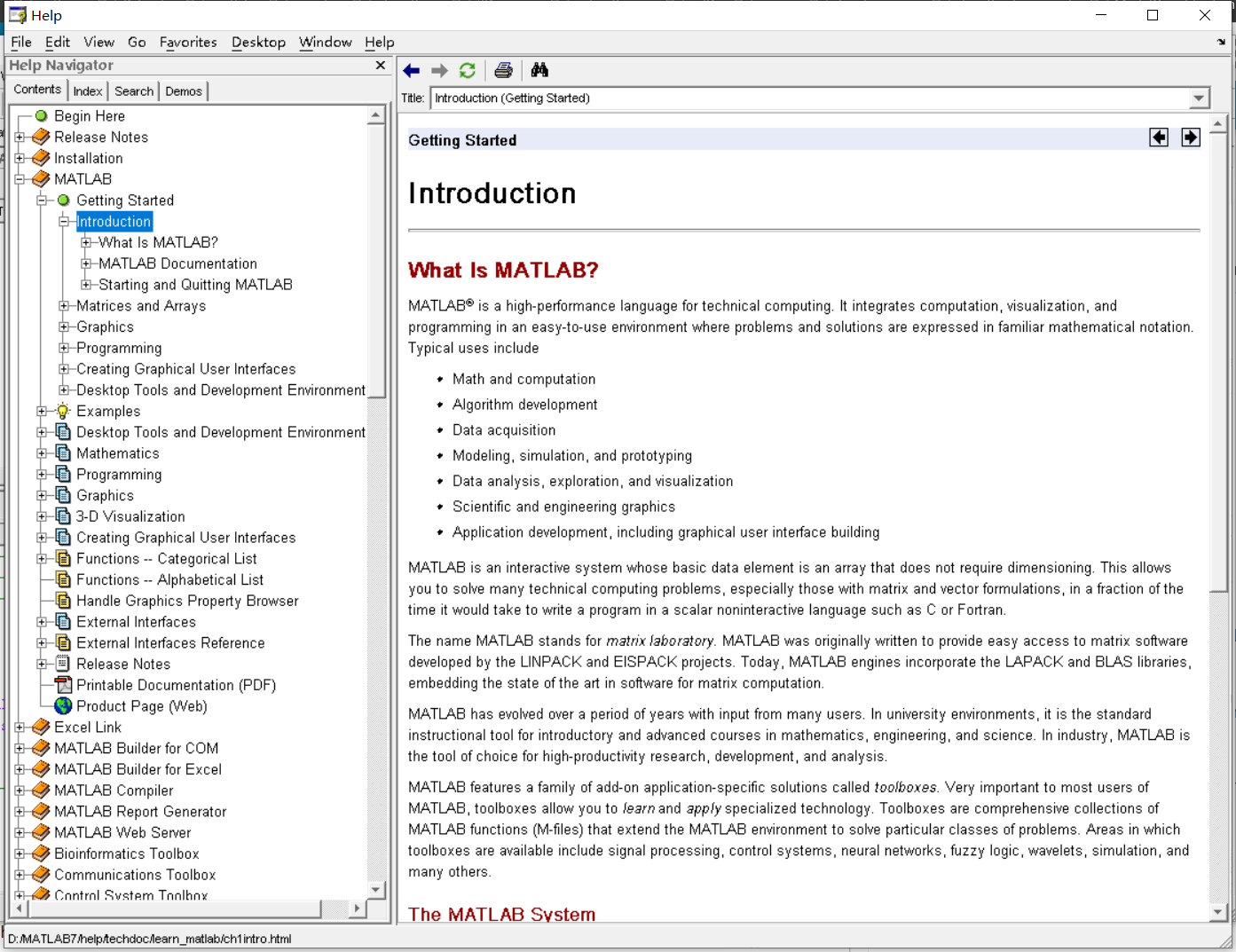
It was 2010 when I was a sophomore in university. I chose to learn MATLAB because of a mathematical modeling competition, and the university provided MATLAB 7.0, a very classic release. To get started, I borrowed many MATLAB books from the library and began by learning simple numerical calculations, plotting, and solving equations. Gradually I was drawn in by MATLAB’s powerful capabilities and became interested; I often used it as a big calculator for fun. That version didn’t have MATLAB Live Script; instead it used MATLAB Notebook (M-Book), which allowed MATLAB functions to be used directly within Microsoft Word, and it also had the Symbolic Math Toolbox’s MuPAD interactive environment. These were later gradually replaced by Live Scripts introduced in R2016a. There are many similar examples...
Out of curiosity, I still have screenshots on my computer showing MATLAB 7.0 running compatibly. I’d love to hear your thoughts?