Results for
I have both of my account profile and channel export time zones set to "(GMT+8000)Beijing". The datetime from the exported feeds.csv looks like:
'2021-09-06 11:16:28 CST'
I want to import data, but MATLAB do not directly understand its datetime format. I assume "CST" to be "China Standard Time", but when I try to convert it to datetime, MATLAB throws an error:
 >> datetime(s,'InputFormat',"yyyy-MM-dd HH:mm:ss z","TimeZone","Asia/Shanghai","Locale","zh_CN")
 Error using datetime (line 651)
 Unable to convert '2021-09-06 11:16:28 JST' to datetime using the format 'yyyy-MM-dd HH:mm:ss z' and locale 'zh_CN'.
However if I change the "Locale" to US instead:
>>datetime(s,'InputFormat',"yyyy-MM-dd HH:mm:ss z","TimeZone","Asia/Shanghai","Locale","en_US")
ans =
    datetime
07-Sep-2021 01:16:28
There is no error, but the time is wrong and is 14 hours ahead. So I guess that MATLAB sees this "CST" as "Central Standard Time".
My point is:
- It's pretty strange that the datetime exported by ThingSpeak could not be directly understood by MATLAB. MATLAB is supposed to work with ThingSpeak data seamlessly, but now I have to find a detour to import ThingSpeak data to MATLAB.
- It seems that the datetime function needs improvement to understand this "CST" timezone, or that ThingSpeak could improve its datetime output format.
New to r2020a, leapseconds() creates a table showing all leap seconds recognized by the datetime data type.
>> leapseconds()
ans =
  27×2 timetable
       Date        Type    CumulativeAdjustment
    ___________    ____    ____________________
    30-Jun-1972     +              1 sec
    31-Dec-1972     +              2 sec
    31-Dec-1973     +              3 sec
    31-Dec-1974     +              4 sec
    31-Dec-1975     +              5 sec
             << 21 rows removed >>
    31-Dec-2016     +             27 sec
Leap seconds can covertly sneak into your data and cause errors that are difficult to resolve if the leap seconds go undetected. A leap second was responsible for crashing Reddit , Mozilla, Yelp, LinkedIn and other sites in 2012.
Detect leap seconds present in a vector of years
% Define a vector of years
t = 2005:2008;
allLeapSeconds = leapseconds();
isYearWithLeapSecond = ismember(t,year(allLeapSeconds.Date));
% Show years that contain a leap second
t(isYearWithLeapSecond)
ans =
        2005        2008
Detect leap seconds present in a vector of months
% Define a vector of months
t = datetime(1972, 1, 1) + calmonths(0:11);
t.Format = 'MMM-yyyy';
allLeapSeconds = leapseconds();
[tY,tM] = ymd(t);
[leapSecY, leapSecM] = ymd(allLeapSeconds.Date);
isMonthWithLeapSecond = ismember([tY(:),tM(:)], [leapSecY, leapSecM], 'rows');
% Show months that contain a leap second
t(isMonthWithLeapSecond)
ans =
  1×2 datetime array
   Jun-1972   Dec-1972
List all leap seconds in your lifetime
% Enter your birthday in mm/dd/yyyy hh:mm:ss format
yourBirthday = '01/15/1988 14:30:00';
yourTimeRange = timerange(datetime(yourBirthday), datetime('now'));
allLeapSeconds = leapseconds();
lifeLeapSeconds = allLeapSeconds(yourTimeRange,:);
lifeLeapSeconds.YourAge = lifeLeapSeconds.Date - datetime(yourBirthday);
lifeLeapSeconds.YourAge.Format = 'y';
% Show table
fprintf('\n Leap seconds in your lifetime:\n')
disp(lifeLeapSeconds)
Leap seconds in your lifetime:
       Date        Type    CumulativeAdjustment     YourAge
    ___________    ____    ____________________    __________
    31-Dec-1989     +             15 sec           1.9587 yrs
    31-Dec-1990     +             16 sec            2.958 yrs
                        << 8 rows removed >>
    30-Jun-2012     +             25 sec           24.456 yrs
    30-Jun-2015     +             26 sec           27.454 yrs
    31-Dec-2016     +             27 sec            28.96 yrs
What is a leap second?
A second is defined as the time it takes a cesium-133 atom to oscillate 9,192,631,770 times under controlled conditions. The transition frequency is so precise that it takes 100 million years to gain 1 second of error [1]. If the earth’s rotation were perfectly synchronized to the atomic second, a day would be 86,400 seconds. But the earth’s rate of rotation is affected by climate, winds, atmospheric pressure, and the rate of rotation is gradually decreasing due to tidal friction [2,3]. Several months before the expected difference between the atomic clock-based time (UTC) and universal time (UT1) reaches +/- 0.9 seconds the IERS authorizes the addition (or subtraction) of 1 leap second (see plot below). Since the first leap second in 1972, all leap second adjustments have been made on the last day of June or December and all adjustments have been +1 second which explains the + signs in the type column of the leapseconds() table.
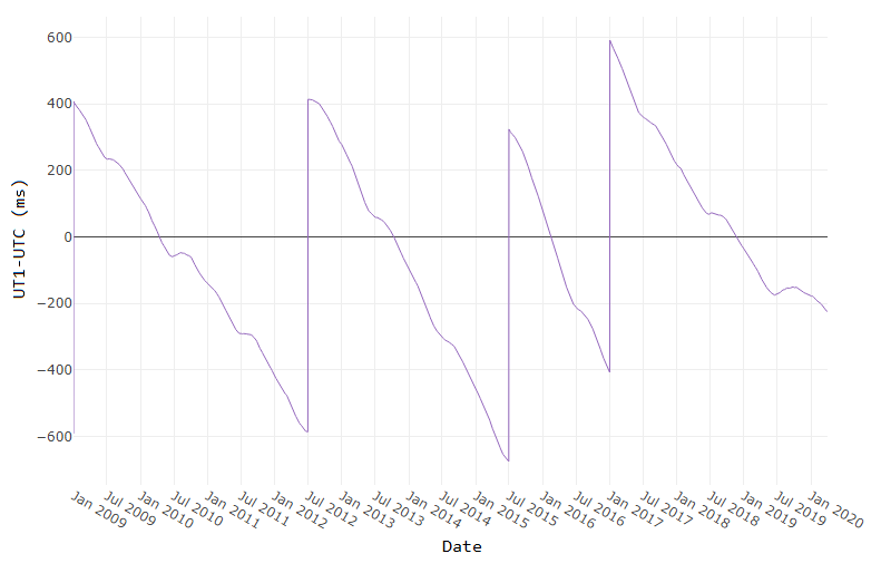
[ Image source ]
How to reference the leap second schedule in your code
Since leap second adjustments are not regularly timed, you can record the official IERS Bulletin C version used at the time of your analysis by accessing the 2nd output to leapseconds().
[T,vers] = leapseconds
What do leap seconds look like in datetime values?
A minute typically has 60 seconds spanning from 0:59. A minute containing a leap second has 61 seconds spanning from 0:60.
December 30, 2016 was a normal day. If we add the usual 86400 seconds to the start of that day, the result is the start of the next day.
d = datetime(2016, 12, 30, 'TimeZone','UTCLeapSeconds') + seconds(86400)
d =
  datetime
   2016-12-31T00:00:00.000Z
The next day, December 31, 2016, had a leap second. If we add 86400 seconds to the start of that day, the result is not the start of the next day.
d = datetime(2016, 12, 31, 'TimeZone','UTCLeapSeconds') + seconds(86400)
d =
  datetime
   2016-12-31T23:59:60.000Z
When will the next leap second be?
As of the current date (April 2020) the timing of the next leap second is unknown. Based on the data from the plot above, what's your guess?
References
Do date ranges from two different timetables intersect?
Is a specific datetime value within the range of a timetable?
Is the range of row times in a timetable within the limits of a datetime array?
Three new functions in r2020a will help to answer these questions.
- [tf, whichRows] = containsrange(TT,__)
- [tf, whichRows] = overlapsrange(TT,__)
- [tf, whichRows] = withinrange(TT,__)
In these function inputs, TT is a timetable and input #2 is one of the following:
- another timetable
- a time range object produced by timerange(startTime,endTime)
- a datetime scalar produced by datetime()
- a duration
The tf output is a logical scalar indicating pass|fail and the whichRows output is a logical vector identifying the rows of TT that are within the specified time range.
How do these functions differ?
Let's test all 3 functions with different time ranges and a timetable of electric utility outages in the United States, provided by Matlab. The first few rows of outages.csv are shown below in a timetable. You can see that the row times are not sorted which won't affect the behavior of these functions.
8×5 timetable
     OutageTime          Region         Loss     Customers     RestorationTime            Cause
  ________________    _____________    ______    __________    ________________    ___________________
  2002-02-01 12:18    {'SouthWest'}    458.98    1.8202e+06    2002-02-07 16:50    {'winter storm'   }
  2003-01-23 00:49    {'SouthEast'}    530.14    2.1204e+05                 NaT    {'winter storm'   }
  2003-02-07 21:15    {'SouthEast'}     289.4    1.4294e+05    2003-02-17 08:14    {'winter storm'   }
  2004-04-06 05:44    {'West'     }    434.81    3.4037e+05    2004-04-06 06:10    {'equipment fault'}
  2002-03-16 06:18    {'MidWest'  }    186.44    2.1275e+05    2002-03-18 23:23    {'severe storm'   }
  2003-06-18 02:49    {'West'     }         0             0    2003-06-18 10:54    {'attack'         }
  2004-06-20 14:39    {'West'     }    231.29           NaN    2004-06-20 19:16    {'equipment fault'}
  2002-06-06 19:28    {'West'     }    311.86           NaN    2002-06-07 00:51    {'equipment fault'}
The range of times in utility.csv is depicted by the gray timeline bar in the plot below labeled "Timetable row times". The timeline bars above it are various time ranges or scalar datetime values used to test the three new functions.
The three columns of checkboxes on the right of the plot show the results of the first output of each function, tf, for each time range.
The time ranges were created by the timerange function using the syntax timerange(startTime,endTime). The default intervalType in timerange() is 'openright' which means that datetimes are matched when they are equal to or greater than startTime and less than but not equal to endTime. The scalar datetime values were created with datetime().
The colorbar along with the colored points at the bottom of each timeline bar show the row numbers of timetable TT that were selected by the whichRows output of the three functions.
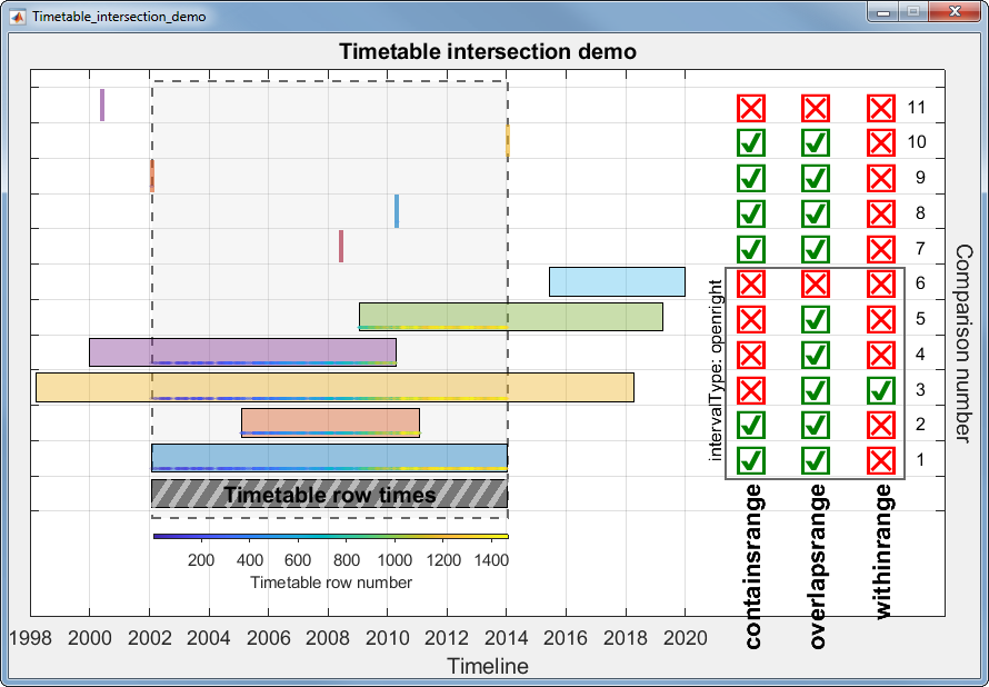
The containsrange() function returns true when all of the time range values are within the timetable including the timetable's minimum and maximum datetime.
The overlapsrange() function returns true when any of the time range values are with the timetable's range.
The withinrange() function returns true only when all of the timetable's datetime values are within the time range values. A careful observer may see that comparison number 1 is false even though that time range is exactly equal to the timetable's row time range. This is because the default value for intervalType in the timerange() function is 'openright' which does not match the end values if they are equal. If you change the intervalType to 'closed' the withinrange result for comparison 1 would be true.
The scalar datetime values for comparisons 8, 9 and 10 are all exact matches of datetimes within the timetable and result in a single match in the whichRows output. The datetime values for comparisons 7 and 11 do not match any of the timetable row times and the values in whichRows are all false even though comparison 7 is within the timetable range. For all three tests, the whichRows outputs are identical.
---------------------------------------------------------------
Here is the code used to generate this data, test the functions, and produce the plot.
% Read in the outage data as a table and convert it to a timetable TT.
T = readtable('outages.csv');
TT = table2timetable(T);
% Look at the first few rows.
head(TT)
% Show that row time vector is not sorted.
issorted(TT)
% Get the earliest and latest row time.
outageTimeLims = [min(TT.OutageTime), max(TT.OutageTime)];
% Define time ranges to test [start,end] or scalar times [datetime, NaT]
% The scalar times must be listed after time ranges.
dateRanges = [ % start, end
    outageTimeLims;                                 % original data
    outageTimeLims;                                 % equal time range
    datetime(2005,2,1), datetime(2011,2,1);         % all within
    datetime(1998,3,16), datetime(2018,4,11);       % starts before, ends after
    datetime(2000,1,1), datetime(2010,4,11);        % starts before, ends within
    datetime(2009,1,15), datetime(2019, 4,7);       % starts within, ends after
    datetime(2015,6,15), datetime(2019,12,31);      % all outside
    datetime(2008,6,6), NaT;                        % 1-value, inside, not a member
    [TT.OutageTime(find(year(TT.OutageTime)==2010,1)), NaT] % 1 value, inside, is a member
    outageTimeLims(1), NaT;                         % 1-value, on left edge
    outageTimeLims(2), NaT;                         % 1-value, on right edge
    datetime(2000,6,6), NaT;                        % 1-value, outside
    ];
nRanges = size(dateRanges,1);
dateRangeLims = [min(dateRanges,[],'all'), max(dateRanges,[],'all')];
% Set up the figure and axes
uifig = uifigure('Name', 'Timetable_intersection_demo', 'Resize', 'off');
uifig.Position(3:4) = [874,580];
movegui(uifig,'center')
uiax = uiaxes(uifig, 'Position', [0,0,uifig.Position(3:4)], 'box', 'on', 'YAxisLocation', 'right',...
    'ytick', -.5:1:nRanges, 'YTickLabel', [], 'ylim', [-3.5, nRanges], 'FontSize', 18);
hold(uiax, 'on')
grid(uiax, 'on')
uiax.Toolbar.Visible = 'off';
% Add axes labels & title
title(uiax, strrep(uifig.Name,'_',' '))
xlabel(uiax, 'Timeline')
ylab = ylabel(uiax, 'Comparison number');
set(ylab, 'Rotation', -90, 'VerticalAlignment', 'Bottom')
% Add the timetable frame
fill(uiax, outageTimeLims([1,2,2,1]), [-.7,-.7,nRanges-.3,nRanges-.3] , 0.85938*[1,1,1], ... %gainsboro
    'EdgeColor', 0.41016*[1,1,1], 'LineStyle', '--', 'LineWidth', 1.5, 'FaceAlpha', .25)     %dimgray
% Set xtick & xlim after x-axis is converted to datetime
range = @(x)max(x)-min(x);
uiax.XLim = dateRangeLims + range(dateRangeLims).*[-.01, .40];
uiax.XTick = dateshift(dateRangeLims(1),'start','Year') : calyears(2) : dateshift(dateRangeLims(2),'start','Year','next');
xtickformat(uiax,'yyyy')
% Set up timeline plot
lineColors = [0.41016*[1,1,1]; lines(nRanges-1)]; %dimGray
uiax.Colormap = parula(size(TT,1));
tfUniCodes = {char(09745),char(09746)}; %{true, false} checkbox characters
barHeight = 0.8;
rightMargin = [max(dateRangeLims),max(uiax.XLim)];
tfCenters = linspace(rightMargin(1),rightMargin(2),5);
tfCenters([1,end]) = [];
intervalType = 'openright';  % open, closed, openleft openright(def);  see https://www.mathworks.com/help/matlab/ref/timerange.html#bvdk6vh-intervalType
% Loop through each row of dateRanges
for i = 0:nRanges-1
    % Plot timeline bar
    pObj = fill(uiax, dateRanges(i+1,[1,2,2,1]), i+[-barHeight,-barHeight,barHeight,barHeight]/2, lineColors(i+1,:), 'FaceAlpha', .4);
      % Evaluate date ranges and single values differently
      if any(isnat(dateRanges(i+1,:)))
          % Test single datetime
          tr = dateRanges(i+1,~isnat(dateRanges(i+1,:)));
          set(pObj, 'LineWidth', 3, 'EdgeAlpha', .6, 'EdgeColor', lineColors(i+1,:))
      else
          % Test date range
          tr = timerange(dateRanges(i+1,1), dateRanges(i+1,2),intervalType);
      end
% Create timerange obj and test for intersections
[tf(1), whichRows{1}] = containsrange(TT,tr);
[tf(2), whichRows{2}] = overlapsrange(TT,tr);
[tf(3), whichRows{3}] = withinrange(TT,tr);
% Confirm that all 'whichRows' are equal
assert(isequal(whichRows{1},whichRows{2},whichRows{3}), 'Unequal whichRows outputs.') if i>0
% Add pass/fail checkboxes
text(uiax, tfCenters(tf), repmat(i,1,sum(tf)), repmat(tfUniCodes(1),1,sum(tf)), ...
'HorizontalAlignment', 'Center', 'Color', [0 .5 0], 'FontSize', 36, 'FontWeight', 'Bold')
% Fail checkboxes
text(uiax, tfCenters(~tf), repmat(i,1,sum(~tf)), repmat(tfUniCodes(2),1,sum(~tf)), ...
'HorizontalAlignment', 'Center', 'Color', [1 0 0], 'FontSize', 36, 'FontWeight', 'Bold') % Plot the TT row number matches
scatter(uiax, TT.OutageTime(whichRows{1}), repmat(i-barHeight/2+.1,1,sum(whichRows{1})), ...
10, uiax.Colormap(whichRows{1},:), 'filled', 'MarkerFaceAlpha', 0.2)
else
% add stripes to reference bar
xHatch = linspace(dateRanges(i+1,1)-days(2), dateRanges(i+1,2)+days(2), 20);
yHatch = repmat(unique(pObj.YData), 1, 19);
plot(uiax, [xHatch(1:end-1);xHatch(2:end)], yHatch, '-', 'Color', [1 1 1 .5], 'LineWidth', 4)
pObj.FaceAlpha = .9;
text(uiax, mean(outageTimeLims), 0, 'Timetable row times', 'FontSize', 20, ...
'HorizontalAlignment', 'Center', 'VerticalAlignment', 'middle', 'FontWeight', 'Bold')
end
end% Draw frame around checkboxs for duration comparisons and label intervalType
rectEdges = linspace(rightMargin(1),rightMargin(2),33);
nDurations = sum(~isnat(dateRanges(:,2)))-1;
fill(uiax, rectEdges([6,end-5,end-5,6]), [.4 .4 nDurations+[.4,.4]], 'w', ...
'FaceAlpha', 0, 'LineWidth', 1.5, 'EdgeColor', 0.41016*[1,1,1]) % dimgray
text(uiax, rectEdges(6), nDurations/2+.5, sprintf('intervalType: %s', intervalType), 'FontSize', 16, ...
'HorizontalAlignment', 'Center', 'VerticalAlignment', 'Bottom', 'Rotation', 90)
% Add text labels for checkboxes and comparison number
text(uiax, tfCenters, [.5 .5 .5], {'containsrange ', 'overlapsrange ', 'withinrange '}, 'Fontsize', 22, 'Rotation', 90, ...
    'HorizontalAlignment', 'right', 'FontWeight', 'b')
text(uiax, repmat(rightMargin(2)-range(xlim(uiax))*.02,1,nRanges-1), 1:nRanges-1, cellstr(num2str((1:nRanges-1)')), ...
    'HorizontalAlignment', 'Right', 'FontSize', 16)
% Add color bar; position it under the timetable bar (must be done after all other axes properties are set)
% requires coordinate tranformation from data units to fig position units.
cb = colorbar(uiax, 'Location', 'South', 'TickDirection', 'Out', 'YAxisLocation', 'Bottom', 'FontSize', 11);
caxis(uiax, [1,size(TT,1)])
cb.Position(3) = range(outageTimeLims)/range(xlim(uiax))  * (uiax.InnerPosition(3)/uifig.Position(3));
cb.Position(1) = ((outageTimeLims(1)-min(xlim(uiax)))/range(xlim(uiax)) * uiax.InnerPosition(3) + uiax.InnerPosition(1)) / uifig.Position(3);
cb.Position(4) = 0.008;
cb.Position(2) = ((-barHeight-min(ylim(uiax))-.5)/range(ylim(uiax)) * uiax.InnerPosition(4) + uiax.InnerPosition(2)) / uifig.Position(4);
ylabel(cb, 'Timetable row number')