Diese Seite wurde maschinell übersetzt.
Füllen Sie bitte eine 1-Minuten-Befragung zur Qualität dieser Übersetzung aus.
Akku-Schnellladung mit Simscape Battery und About:Energy
Von Darryl Doyle und Yashraj Tripathy, About:Energy; Steve Miller und Sebastián Arias, MathWorks
Die Integration von About:Energy TSPMe und elektrischen Modellen mit detaillierten Packmodellen auf Basis von Simscape Battery gewährleistet Genauigkeit und Sicherheit in Batteriemanagementsystemen und unterstützt laufende Fortschritte im Bereich des Batterieladens.
Die Schnellladezeit der Batterie ist ein entscheidender Leistungsindikator bei der Konstruktion von Elektrofahrzeugen (EVs) und ein Hauptanliegen der EV-Kunden. Dieser Artikel zeigt, wie Sie mit Simscape Battery™ sowie benutzerdefinierten Zellmodellblöcken und Parametern, die von About:Energy entwickelt wurden, sichere und robuste Schnellladeprofile für verschiedene Batteriesystemgrößen erstellen. Hierzu gehören DC-Batterie-Schnellladeprofile der Stufe 1 (bis zu 80 kW) und der Stufe 2 (bis zu 400 kW, auch als Stufe 3 bezeichnet) gemäß SAE J1772. Dieser Artikel zeigt auch, wie Sie mit Simscape™ und dem Battery Pack Builder-Workflow von Simscape Battery benutzerdefinierte Batteriezellenmodelle skalieren (Abbildung 1).

Abbildung 1. Schnelllade-Workflow von der Zelle zum Akkupack mithilfe benutzerdefinierter Simscape Zellenmodellblöcke im Battery Builder.
Mehrere Prozesse innerhalb einer Lithium-Ionen-Batteriezelle für Elektrofahrzeuge beeinflussen die maximale Ladegeschwindigkeit der Zelle, beispielsweise die Lithiumdiffusion in der negativen Elektrode und der Lithium-Ionen-Transport im Elektrolyt. Diese Prozesse finden auf mikroskopischer Ebene statt und werden von der lokalen Temperatur, dem Ladezustand (SOC) und Gesundheitszustand (SOH) der einzelnen Batteriezellen sowie der Zellchemie bestimmt. Auf der Ebene der Batteriemodule und -pakete spielen auch noch andere Faktoren eine Rolle, wie etwa die Stromgrenzen des Systems und des Gleichstromladegeräts, Temperaturunterschiede zwischen den Zellen aufgrund der Wärmemanagementstrategie, SOC-Schwankungen aufgrund des elektrischen Designs, der Steuerungsstrategie, der Sensorplatzierung, des elektrischen Widerstands außerhalb der Zelle und der Fertigungsvariabilität. Diese zusätzlichen Faktoren können die Schnellladegeschwindigkeit noch weiter einschränken. Daher ist es wichtig, alle diese Variablen bei allen Batteriedesign- und Validierungsabläufen zu berücksichtigen.
Batteriezellenmodelle
Die Battery Builder-Funktionalität in Simscape Battery ermöglicht die automatisierte Erstellung von Batteriemodul- und Packmodellen aus benutzerdefinierten Simscape Blöcken einer einzelnen Batteriezelle, einschließlich der von About:Energy bereitgestellten Batteriezellenblöcke. In diesem Artikel zeigen wir zwei Arten von zuvor validierten Batteriemodellen einer nickelreichen, hochenergetischen 2170-Zelle, die von About:Energy bereitgestellt wurden:
- Ein thermisches Einzelpartikelmodell mit Elektrolyt (TSPMe), das Zugriff auf interne elektrochemische Zustände oder Variablen bietet, die für die Durchführung von Aufgaben wie der Schnellladesteuerung erforderlich sind.
- Ein speziell für die Schnellladung parametriertes Ersatzschaltbildmodell (ECM), das nach der Skalierung auf Modul- oder Packebene relativ schnellere Rechenzeiten bietet.
Die Simscape Battery Bibliothek enthält auch Modellblöcke für Batteriezellen, die den Ersatzschaltbildansatz und ein elektrochemisches Einzelpartikelmodell verwenden (Abbildung 2). Diese sind in Simscape Battery seit R2023b und R2024a verfügbar.

Abbildung 2. Grundlegende Batteriezellenmodellblöcke in Simscape.
Ausgearbeitetes Beispiel von der Zelle zum Modul
Mithilfe der Batterieerstellungsfunktion in Simscape Battery können wir schnell Prototypen von Batteriesystemmodellen erstellen und die Schnellladezeiten von Batterien für verschiedene Unterkomponentenebenen unter einer breiten Palette thermischer und elektrischer Randbedingungen und anfänglicher Betriebszustände (SOC und Temperatur) bewerten.
Zuerst müssen wir ein Batteriezellenobjekt definieren und dieses Zellobjekt mit dem entsprechenden Zellmodellblock verknüpfen, der von About:Energy bereitgestellt wird. Wir skalieren zuerst das ECM hoch. Um den ECM-Block zu verwenden, laden wir zunächst elektrothermische Parameter, die von About:Energy bereitgestellt werden und in einer Struktur namens cellData.
run("CellModelParameters.mlx") % Load cell ECM parameters (e.g., capacity, energy)
Um das Batteriezellenobjekt zu definieren, müssen wir die Cell-Klasse aus dem Battery Builder-Paket in Simscape Battery wie folgt instanziieren:
import simscape.battery.builder.* % Import battery builder package

battCell = Cell(Geometry = CylindricalGeometry(...
    'Height',simscape.Value(cellData.cellHeight,'m'),...
    'Radius',simscape.Value(cellData.cellRadius,'m')), ...
    Capacity = simscape.Value(cellData.cellCapacity,"A*hr"), ...
    Energy = simscape.Value(cellData.cellNominalEnergy,"W*hr")); % Cell object
Wir können unser Batteriezellenobjekt mit benutzerdefinierten About:Energy-Blöcken verknüpfen, indem wir die CellModelOptions Eigenschaft wie folgt modifizieren:
battCell.CellModelOptions.CellModelBlockPath = "AE_Mathworks_lib/AE_mathworks_ECM";
disp(battCell.CellModelOptions)

CellModelBlock with properties:

CellModelBlockPath: "AE_Mathworks_lib/AE)_mathworks_ECM"
    BlockParameters: [1x1 struct]
Für dieses Beispiel erstellen wir eine 400-Volt-Traktionsbatterie im Automobilstil, die aus 16 Batteriemodulen besteht. Jedes Batteriemodul besteht aus 36 zylindrischen Zellen, die elektrisch parallel geschaltet sind, und dann sechs dieser parallelen Baugruppen, die elektrisch in Reihe geschaltet sind (36p6s). Der Code zum Hochskalieren der Zellkomponente in eine parallele Baugruppe und dann in ein Modul wird unten angezeigt:
battPSet = ParallelAssembly(Cell = battCell, NumParallelCells = 36,...
    Rows = 9, ModelResolution="Detailed",...
    NonCellResistance = "on",...
    AmbientThermalPath="CellBasedThermalResistance", ...
    CoolantThermalPath="CellBasedThermalResistance",...
    CoolingPlate="Bottom"); % Parallel assembly object

battModule = Module(ParallelAssembly = battPSet, NumSeriesAssemblies = 6,...
    NonCellResistance = "on",...
    ModelResolution="Grouped",...
    SeriesGrouping = [1,4,1],...
    ParallelGrouping = [36,1,36],...
    AmbientThermalPath="CellBasedThermalResistance", ...
    CoolantThermalPath="CellBasedThermalResistance",...
    CoolingPlate="Bottom"); % Module object
Alternativ können wir dasselbe Batteriedesign und dieselben Objekte auch mit der App „Battery Builder“ definieren (Abbildung 3).

Abbildung 3. Die App-Schnittstelle Battery Builder für den Batterieentwurf.
Wir können automatisch Simscape Modelle aus den oben definierten Batterieobjekten generieren, indem wir den buildBattery-Funktion. Beim Aufruf dieser Funktion können wir auch das MaskParameters Name-Wert-Paar auf „VariableNamesByType “ setzen, um ein Skript mit allen zum Ausführen des Modells erforderlichen Parametern zu generieren. Vor der Modellerstellung können wir unsere Batteriedefinition und unser Design überprüfen, indem wir das BatteryChart-Objekt nutzen, das hilft, die Geometrie und Positionierung der Batteriezellen in einem 3D-Raum zu visualisieren. Tabelle 1 zeigt die typischen Ausgaben aus der Verwendung dieser Funktionen für unsere Modul- und Parallelassemblierungsobjekte.
| Batterievisualisierungscode | Code zur Erstellung eines Batteriemodells |
f = uifigure(Color="w");
BatteryChart(Battery=battPSet);

|
buildBattery(battPSet, Library= "detailedPSet",... MaskParameters = "VariableNamesByType"); 
|
f = uifigure(Color="w");
BatteryChart(Battery=battModule);

|
buildBattery(battModule, Library= "groupedModule",... MaskParameters = "VariableNamesByType"); 
|


Als Nächstes definieren wir die elektrische Schnellladelast, die zum Testen der generierten Batteriemodelle verwendet wird. Um dies zu erreichen, müssen wir zunächst die Schnellladefähigkeit der Batteriezelle abschätzen.
Schnelles Laden auf Zellebene
Bei einem Schnellladevorgang besteht je nach Betriebsbedingungen der Batterie und ihrer Elektrochemie ein höheres Risiko einer Lithium-Plating-Verursachung. Die wichtigste treibende Kraft hinter der Lithiumbeschichtung ist letztendlich der lokale Potenzialunterschied zwischen der festen und der flüssigen Phase an der Anoden-Elektrolyt-Grenzfläche, der von vielen Faktoren beeinflusst wird, wie etwa Temperatur, Diffusionsbeschränkungen, SOC und Laderate. Kalte Temperaturen führen generell zu trägen Transportvorgängen und größeren Potentialunterschieden beim Laden. Daher führen Temperaturunterschiede innerhalb der Zelle und Unterschiede im SOC natürlich dazu, dass in verschiedenen Bereichen der Zelle das Risiko einer Lithium-Plating-Infektion steigt. Diese Unterschiede sind bei einem bestimmten Zelldesign und den thermischen Randbedingungen rund um die Zelle immer vorhanden. Tabelle 2 zeigt die wichtigsten internen Variablen und Randbedingungen, die zur Erstellung eines sicheren und schnellen Ladeprofils berücksichtigt werden müssen.
| Variable | Beschreibung und Code |
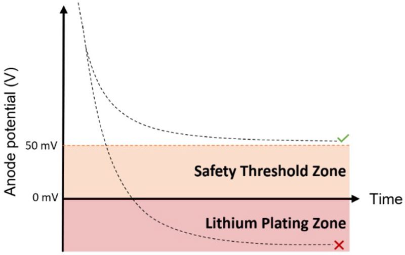
| Anodenpotential | Wir verwenden das elektrostatische Potenzial der negativen Elektrode in Bezug auf eine Li/Li+-Referenzelektrode als Indikator für ein erhöhtes Risiko einer Lithiumablagerung und einer beschleunigten Degradation. Beim Laden sinkt dieses Potenzial aufgrund des Massentransports und der chemischen Reaktionsprozesse im Inneren der Zelle. Um das Risiko einer Lithium-Plating-Erkrankung zu verringern, darf dieses Potenzial nicht zu weit unter 0 V fallen. In diesem Beispiel wird dieser Potenzialschwellenwert willkürlich auf 50 mV festgelegt.

AnodePotentialThreshold = 0.05; % Unit: V
|
| Batterietemperatur | Die Zelltemperatur muss unterhalb ihrer Betriebsgrenze bleiben, um die Degradation zu begrenzen und das Risiko eines thermischen Durchgehens zu verringern. TemperatureThreshold = 55 + 273.15; % Unit: K
|
| Anfängliche Batterietemperatur | Höhere Temperaturen ermöglichen höhere Ströme. Wenn die maximale Betriebstemperatur erreicht wird, reduziert das Steuersystem den Strom und verlängert die Ladezeit. Niedrigere Anfangstemperaturen bieten ein größeres Temperaturdelta zur Dämpfung der hohen Wärmeentwicklung, jedoch begrenzen niedrigere Temperaturen auch den maximalen Strom. Daher gibt es eine optimale Anfangstemperatur, die durch Simulation oder physikalische Tests ermittelt werden kann. InitialCellTemperature = 35 + 273.15; % Unit: K
|
| Randbedingungen des Wärmemanagements | In diesem Beispiel betrachten wir eine „von unten gekühlte“ Batteriezelle, die in eine Kühlplatte eingegossen ist, wie im folgenden Diagramm dargestellt. Wir gehen von einem konstanten Wärmewiderstand von 5 K/W aus, der von der Zellbodenoberfläche bis zum Kühlmittel im Kühlkanal definiert ist.
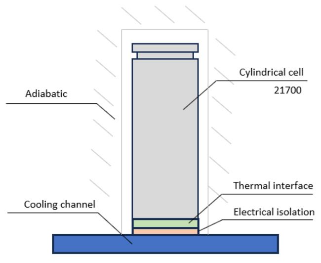
CellThermalPathResistance = 5; % Unit: K/W
|
| Batterieklemmenspannung | Während des Ladevorgangs steigt die Zellspannung an. Um Überspannungs- oder Überladungszustände zu vermeiden, kann die Batteriespannung den vom Zellenlieferanten angegebenen Höchstwert nicht überschreiten. MaximumBatteryVoltage = 4.2; % Unit: V
|
| Vollständig aufgeladener Akku | Am Ende der Ladephase steigt die Klemmenspannung auf ihren Maximalwert. Um eine optimale Schnellladung zu gewährleisten und Überladungszustände zu vermeiden, muss der Strom in einem konstanten Spannungsschritt (CV) reduziert werden. In diesem Artikel ist der vollständig geladene Zustand (100 % SOC) erreicht, sobald der Stromwert unter 1/10 der Nennkapazität der Zelle fällt. FullyChargedCurrentThreshold = cellData.cellCapacity/10; % Unit: A
|
| Maximaler Ladestrom | Dieser Wert sollte vom Batteriehersteller für einen bestimmten Satz von Bedingungen (SOC, SOH, Temperatur) angegeben werden. Im Allgemeinen können Batterien für kurze Zeit höhere Ladeströme und für längere Zeit geringere Ladeströme aufnehmen. MaximumChargeCurrent = 30; % @ 0% SOC, instantaneous limit, Unit: A
|

Schnellladeprofil-Methodik
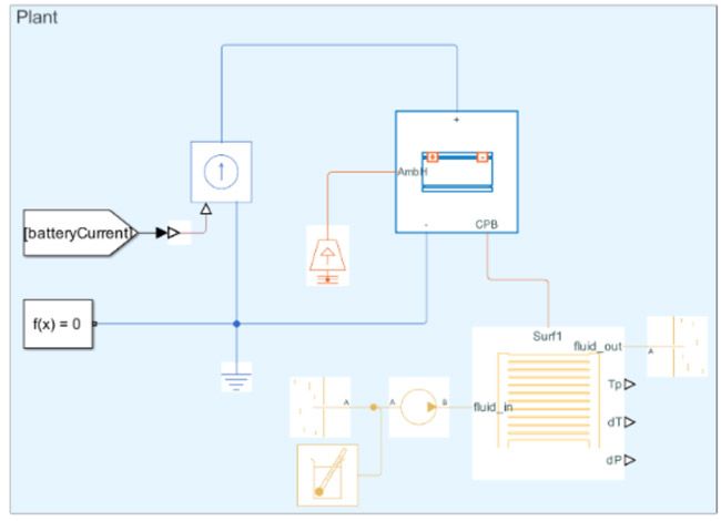
Um das Anodenpotential über die gesamte Biskuitrolle hinweg zu überwachen, wurde ein höhendiskretisiertes elektrothermisches Zellebenenmodell erstellt. Als Grundlage wurde die Programmiersprache Simscape und das About:Energy TSPMe-Modell verwendet (Abbildung 4). Das thermische Modell wird entlang der Höhe diskretisiert, um die thermischen Gradienten zu erfassen, die durch die Basiskühlung entstehen. Die diskretisierten Elemente sind elektrisch parallel und thermisch in Reihe geschaltet, sodass das Zellinnere nachgebildet wird und eine höhere interne Zustandsauflösung möglich ist. Durch eine zusätzliche radiale Aufteilung der Elemente lassen sich höhere und genauere Zustandsauflösungen erreichen. About:Energy bietet außerdem 2D-Wärmemodellblöcke von Simscape.

Abbildung 4. Diskretes Batteriezellenmodell, erstellt mit Simscape und Simulink.
Drei PI-Regler drosseln den maximal zulässigen Strom und sorgen für sichere Betriebsbedingungen (Abbildung 5):

Abbildung 5. Simulink Steuerungsstrategie für das diskretisierte Batteriezellenmodell.
Die Ableitung des optimalen Ladestroms erfolgt nach folgender Strategie (Abbildung 6):
- Laden der Batterie mit der schnellsten vom Lieferanten zugelassenen Rate bei 0 % SOC und der ausgewählten Anfangstemperatur.
- Reduzieren des Stroms, wenn das Anodenpotential seinen angegebenen Schwellenwert erreicht.
- Reduzieren, wenn die heißeste Stelle der Batteriezelle die maximale Betriebstemperatur erreicht.
- Reduzieren, um eine Überladung zu verhindern, wenn die Klemmenspannung die maximale Spannungsgrenze erreicht.
- Fügen Sie bei Bedarf weitere Derating-Bedingungen hinzu, die sich an andere Zustände, wie etwa die Lithiumkonzentration im Elektrolyt, richten.
- Der Ladevorgang wird beendet, sobald die konstante Spannungsstufe C/10 erreicht.
- Speichern Sie das zuletzt gelieferte Stromsignal als Ihr endgültiges Schnellladestromprofil.
cellSimulation = sim("CellLevelFastCharge.slx","StartTime","0","StopTime","3600");
run("PlotCellSimulation.mlx");

Abbildung 6. Ergebnisse aus der diskreten Batteriezellenmodellsimulation.
Tabelle 3 fasst die diskretisierten Simulationsergebnisse auf Zellenebene unter Berücksichtigung unserer Annahmen zusammen.
| SOC-Fenster | Schnellladezeit (in Min) | Bedingungen |
| 0–80 % | 14. | @ 35 °C Anfangstemperatur, BoL und angenommene Einschränkungen |
| 0–100 % | 30 | @ 35 °C Anfangstemperatur, BoL, C/10 CV-Bedingung |
Karte zum schnellen Aufladen von Zellen
Der im vorherigen Abschnitt erstellte Schnellladeregler gibt ein Stromprofil aus, das nur für die angenommene Anfangstemperatur und den angenommenen Anfangs-SOC gültig ist und Ungleichmäßigkeiten in den Anfangs- oder dynamischen Werten dieser Zustände nicht berücksichtigt. Wir können eine allgemeinere zweidimensionale Karte des maximalen Ladestroms als Funktion der Temperatur und des SOC (zu Beginn der Lebensdauer) ableiten, indem wir mehrere Simulationen bei unterschiedlichen Anfangsbedingungen ausführen.
Mithilfe von Stateflow®-Logik können wir für jeden Satz von Anfangsbedingungen eine Simulation ausführen, bei der wir den Strom schnell von null Ampere erhöhen, bis wir den Schwellenwert des Anodenpotentials oder den Schwellenwert der Klemmenspannung erreichen (Abbildung 7). Wenn einer dieser Schwellenwerte erreicht wird, drosseln wir den Strom, um die Begrenzungsvariable für eine bestimmte Dauer konstant bei ihrem Schwellenwert zu halten. In diesem Artikel wird diese Dauer willkürlich auf 60 Sekunden festgelegt (manchmal auch als kontinuierliches Limit bezeichnet), um ein Ereignis von langer Dauer, wie etwa einen Ladevorgang, zu simulieren.

Abbildung 7. Diskrete Batteriezellenmodellsimulation zur Ermittlung der Zellladestromgrenzen.
Im Allgemeinen führen längere Zeiträume zu niedrigeren oder restriktiveren Stromgrenzwerten. Die Simulation stoppt im angegebenen Zeitrahmen und dann speichern wir den endgültigen aktuellen Wert als Grenzwert (Abbildung 8). Die resultierende Karte kann als Eingabe für unsere zuvor definierten Simulationen auf Systemebene verwendet werden, die keinen Zugriff auf die internen elektrochemischen Zustände wie die Anodenpotentiale haben.
InitialCellTemperatureVector = [5,15,25,35,45,50] + 273.15; % Unit: K
InitialSOCVector = [0,0.05,0.1,0.2,0.5,0.6,0.8,0.95]; % Unit: -

for initTempIdx = 1:numel(InitialCellTemperatureVector)
    for initSOCIdx = 1:numel(InitialSOCVector)
        InitialCellTemperature = InitialCellTemperatureVector(initTempIdx);
        InitialSOC = InitialSOCVector(initSOCIdx);
        cellSimulations(initTempIdx).SOCPoint(initSOCIdx).Data = sim("CellLevelFastChargeLimitsStateFlow.slx","StartTime","0","StopTime","60");
        cellCurrentLimit(initTempIdx,initSOCIdx) = cellSimulations(initTempIdx).SOCPoint(initSOCIdx).Data.simout.Data(end);
        save cellCurrentLimit
    end
end

newCellCurrentLimit = [cellCurrentLimit, zeros(1,numel(cellCurrentLimit(:,1)))'];

figure("Color","w")
[xq,yq]= meshgrid([5:1:50]+273.15, 0:0.05:1);
vq = griddata(InitialCellTemperatureVector,[InitialSOCVector,1],newCellCurrentLimit',xq,yq);
mesh(xq,yq,vq)
xlabel('Temperature (°C)')
ylabel('State of Charge (-)')
zlabel('Current Limit (A)')
view([-5 3.5 5])

Abbildung 8. Kontinuierliche Ladestrombegrenzungskarte als Funktion von Temperatur und SOC.
Schnelles Laden auf Parallel-Verbund-Ebene
Bei der Herstellung von Batteriepacks für Elektrofahrzeuge wird eine Batteriezelle typischerweise zunächst elektrisch parallel zu anderen Zellen verbunden, um eine Parallelanordnung zu bilden und so die Batteriekapazität und -energie zu erhöhen. Um das Schnellladeprofil für ein parallel montiertes Subsystem zu berechnen, müssen wir einfach das erhaltene Schnellladeprofil der Zelle mit der Anzahl der parallel geschalteten Zellen multiplizieren. Abhängig von dieser Zahl P könnte der resultierende Schnellladestrom die maximale Stromgrenze der an Ladestationen vorhandenen üblichen Gleichstromladegeräte überschreiten. Dies ist eine wichtige Einschränkung, die Sie bei der Vorhersage von Schnellladezeiten auf Systemebene berücksichtigen müssen.
Bei einer bestimmten Batterieenergie und einer festen Gesamtzahl von Zellen verfügen 400-Volt-Batteriepacks typischerweise über eine höhere Anzahl parallel geschalteter Zellen als 800-Volt-Systeme. Wenn wir das im ersten Abschnitt hergeleitete optimale Zell-Schnellladeprofil nutzen möchten, ergibt sich daraus, dass eine höhere Anzahl parallel geschalteter Zellen zu höheren Schnellladeströmen führt. Für typische 400-Volt-Systeme sind höhere Ströme oder P-Zahlen bedeuten, dass sie eher durch die Ladestation eingeschränkt werden (beim Starten des Ladevorgangs bei 0 % SOC). Diese Einschränkung kann dazu führen, dass die Schnellladefähigkeit der Zelle ungenutzt bleibt und die Ladegeschwindigkeit langsamer ist. Tabelle 4 zeigt typische Maximalströme für verschiedene DC-EV-Ladegeräte.
| Typische externe Ladegerätleistung | Typischer maximaler Dauerstrom |
| 100 kW | 100–250 A |
| 350 kW | 350–500 A |
Abbildung 9 zeigt die Strombegrenzung des Kompressors von 500 Ampere im Vergleich zu typischen, vergrößerten Schnellladeprofilen auf Parallelanordnungsebene für typische 400-Volt- und 800-Volt-Systeme. Da eine höhere Anzahl parallel geschalteter Zellen mit 400-Volt-Systemen zusammenhängt (bei gleicher Batterieenergie), definieren wir willkürlich eine „36 P“-Parallelanordnung stellvertretend für ein 400-Volt-System. Dann vergleichen wir dieses System mit einer „18 P“-Parallelanordnung, repräsentativ für ein 800-Volt-System bei 35 °C.
run("parallelAssemblyProfile.m")

Abbildung 9. Vergleich zwischen 800 V und 400 V Ladeprofilen für 35 °C.
Wie in der Grafik dargestellt, kann das 400-Volt-System zunächst nicht die gesamte Ladekapazität der Zelle nutzen, was zu längeren Ladezeiten als den prognostizierten 0–80 % in 14 Minuten führen kann.
Im Allgemeinen wird die Laderate einer elektrisch verbundenen Batteriegruppe durch den kältesten Punkt an der kältesten Zelle und den Punkt mit dem höchsten SOC innerhalb der Zelle mit dem höchsten SOC bestimmt. Daher basiert die Schnellladesteuerung auf der minimalen Zelltemperatur und den höchsten SOC-Signalen, die vom Modell der parallelen Montageanlage abgerufen werden.
Batteriezellen werden typischerweise auf einem Wärmeleitmaterial ausgelegt, das mit der Kühlplatte in Kontakt steht (die auch eine Schicht zur elektrischen Isolierung enthält). Wir definieren eine zufällige Variation in diesem Wärmepfad, indem wir gewisse Ungleichmäßigkeiten annehmen (z. B. Anwendung von Wärmeleitmaterial zwischen Zellen und einer Kühlplatte).
ParallelAssembly1.CoolantResistance = 14 + (30-14)*rand(36,1)'; % Wärmepfadwiderstand des Kühlmittels auf Zellebene, K/W
Weitere wichtige Aspekte, die mit Simscape modelliert werden können, in diesem Artikel jedoch nicht explizit behandelt werden:
- Innenwiderstand von Zelle zu Zelle und Kapazitätsschwankungen aufgrund der Zellherstellung.
- Bei unsachgemäßer Konstruktion der Kollektorplatte kann es zu leichten Stromungleichgewichten kommen.
- Unterschiedliche Wärmepfade zur Umgebung (diese Dynamik ist normalerweise langsamer).
- Kühlmittelregelung: Normalerweise verfügen Elektrofahrzeuge über einen festen Kühler oder eine Kühlleistung (z. B. 5 kW) zur Wärmeabfuhr aus dem Batteriesystem (und anderen Komponenten). Eine realistische Kühlmittelregelung wirkt sich auch erheblich auf die Schnellladezeit der Batterie aus.
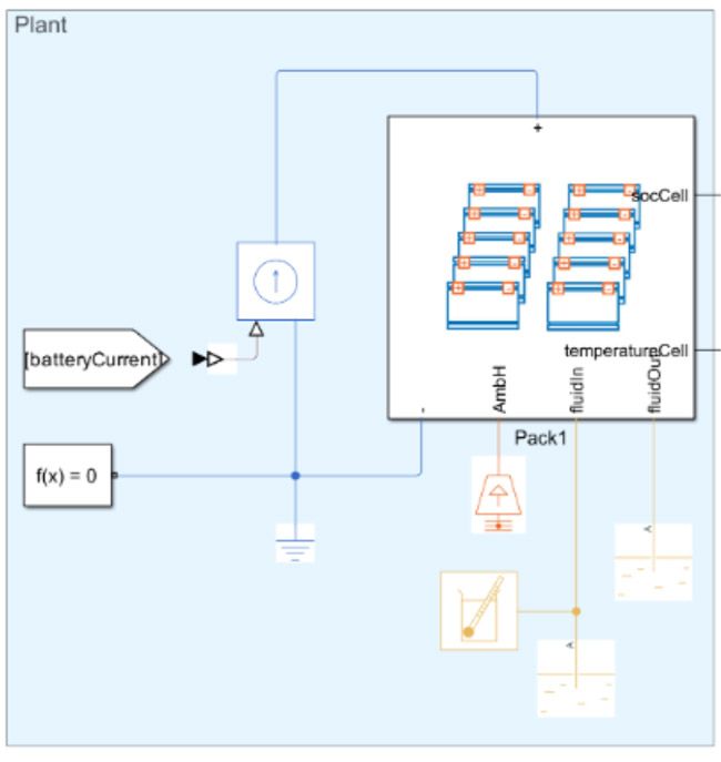
Wir können unseren Parallelverbundblock in Simulink integrieren® und die vergrößerte 2D-Ladungskarte hinzufügen, die wir gerade mit der elektrochemischen Fähigkeit der Zelle abgeleitet haben. Wir haben außerdem einen PI-Regler hinzugefügt, um die maximale Zelltemperatur in der Parallelanordnung zu begrenzen (Abbildung 10).


Abbildung 10. Parallel-Verbund-Simulation (oben) und Parallelmontage-Schnellladeprofil-Steuerblock (unten).
Führen Sie die Parallel-Verbund-Simulation aus und stellen Sie die Ergebnisse grafisch dar (Abbildung 11).
run("detailedPSet_param.m");
set_param("ParallelAssemblyLevelFastCharge","SimscapeLogType",'all')
pSetSimulation = sim("ParallelAssemblyLevelFastCharge.slx","StartTime","0","StopTime","5200");
run("PlotParallelAssemblySimulation.mlx"); % Ergebnisse plotten

Abbildung 11. Ergebnisse der Parallel-Verbund-Simulation.
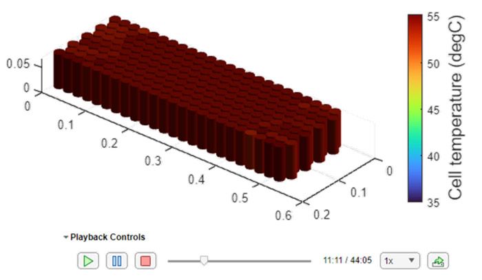
Wie in der Übersichtsdarstellung gezeigt, ist die Parallelanordnung zu Beginn der Simulation durch den Maximalstrom des Ladegeräts von 500 Ampere eingeschränkt. Darüber hinaus erreicht die heißeste Zelltemperatur 55 °C, was zu einer thermischen Leistungsminderung führt, die die Simulationszeit verlängert. Um die dynamischen Temperaturen der Batterie zu visualisieren, können wir ein Batteriesimulationsprotokollobjekt erstellen, wie im folgenden Code gezeigt (Abbildung 12).
pSetSimLog = BatterySimulationLog( battPSet, pSetSimulation.simlog.ParallelAssembly1);
pSetSimLog.SelectedVariableUnit = "degC";
f = uifigure("Color","w");
g = uigridlayout(f, [1,1]);
parallelAssemblyChart = BatterySimulationChart(Parent = g, ...
    BatterySimulationLog = pSetSimLog);
parallelAssemblyChartColorBar = colorbar(parallelAssemblyChart);
ylabel( parallelAssemblyChartColorBar, strcat("Cell temperature", " (", pSetSimLog.SelectedVariableUnit,")") ,'FontSize',14 );
parallelAssemblyChartColorBar = colormap(parallelAssemblyChart);

Abbildung 12. Ergebnisse für dynamische Simulation des Parallelverbunds in BatteryChart.
Wie im dynamischen Batteriediagramm gezeigt, besteht zwischen den Zellen ein Temperaturunterschied von ungefähr 5 °C. Der Unterschied ist hauptsächlich auf die zufällige angenommene Variation des Wärmepfads zum Kühlmittel zurückzuführen. Tabelle 5 zeigt die Ergebnisse der parallelen Montagesimulation. Die Schnellladezeiten von 0–80 % SOC haben sich hauptsächlich aufgrund von Beschränkungen auf Systemebene und thermischen Annahmen um 10 Minuten erhöht.
| SOC-Fenster | Schnellladezeit (min) | Bedingungen |
| 0–80 % | 24 | @ 35 °C Anfangstemperatur, BoL |
| 0–100 % | 43 | @ 35 °C Anfangstemperatur, BoL, C/10 CV-Bedingung |
Richtlinien für benutzerdefinierte Zellblöcke bis R2024a
Der Simscape Battery Pack Builder bietet einige Richtlinien für die effektive Verwendung benutzerdefinierter Zellblöcke:
- Das benutzerdefinierte Zellenmodell darf keine Variable namens
power_dissipatedenthalten. - Wenn thermische Effekte erforderlich sind, muss das Modell mindestens einen Port oder Knoten vom Typ „thermal domain (Thermische Domäne)“ haben.
- Wenn eine Schlüsselvariable eines Zellmodellblocks im Simulink Canvas sichtbar sein muss (z. B. mithilfe des Probe-Blocks), muss diese Variable öffentlich sein, ohne Einschränkungen für
ExternalAccess. Andernfalls ist die Variable nur zur Nachbearbeitung im Simulationsprotokoll sichtbar.
Simulationen vom Modul bis zum Akkupack
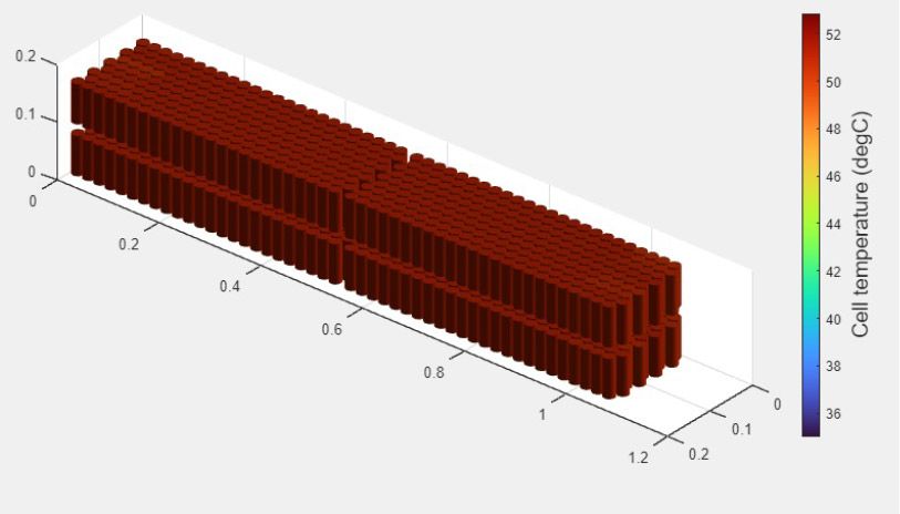
Mit dem gleichen Verfahren wie oben können wir Simulink Modelle für den oben generierten Modulblock und für größere Batterieblöcke, wie z. B. ein Pack, erstellen. Dann können wir diese Blöcke mit demselben parallelen Ladesteuerungsblock koppeln, der auf der 2D-Zellladekarte basiert. Tabelle 6 enthält eine Zusammenfassung dieser Simulationen. Generell erhöht sich die Schnellladezeit bei den aktuellen Modul- und Packdesigns aufgrund größerer Temperaturspannen und höherer Temperaturen an einigen Zellen geringfügig.
| Modell | Ergebnisse/Dynamisches Batteriediagramm |

|
0–80 %: 25 Minuten

|
|
0–80 %: 27 Min.

|

Schlussfolgerungen
- Unsere Untersuchung der Schnellladezeiten von Batterien mithilfe der Blöcke und Parameter aus Simscape Battery und About:Energy hat die Bedeutung eines methodischen mehrskaligen Ansatzes von der Modellierung einzelner Zellen bis hin zu Batteriepacksimulationen gezeigt. Wir betonen, wie wichtig es ist, About:Energy TSPMe und elektrische Modelle mit detaillierten Packmodellen zu integrieren, die durch Simscape Battery ermöglicht werden, um die Genauigkeit und Sicherheit in Batteriemanagementsystemen zu gewährleisten und die laufenden Fortschritte auf dem Gebiet des Batterieladens zu unterstützen. Die größten Unsicherheiten im Zusammenhang mit diesen prognostizierten Schnellladezeiten beruhen vor allem auf der Modellauflösung (z. B. elektrothermische Diskretisierung), den Modellannahmen und der Genauigkeit des verwendeten elektrochemischen/ECM-Modells. Im Allgemeinen führt eine höhere Modelldiskretisierung oder Auflösung zu genaueren Ergebnissen.
- Wie der Workflow von der Zelle zum Batteriepack zeigt, hängen Schnellladezeiten von Batterien von einer Vielzahl von Variablen ab und das Design der Batteriepacks kann einen erheblichen Einfluss haben. Beginnen wir auf Zellebene: Die schnellste Ladegeschwindigkeit einer Batteriezelle hängt von den Diffusions- und Transportprozessen des Lithiums ab, die im kleinen Maßstab stattfinden. Auf Modul- und Packebene werden andere Variablen wichtig, wie beispielsweise die Strombegrenzung des DC-Ladegeräts, die Anzahl parallel geschalteter Zellen, die Nennspannung des Batteriepacks (400 Volt gegenüber 800 Volt), Temperaturschwankungen innerhalb und zwischen Zellen, SOC-Schwankungen innerhalb und zwischen Zellen, Nicht-Zell-Widerstand und andere. Wie in diesem Artikel gezeigt wird, können diese Variablen, insbesondere Temperaturunterschiede, erhebliche Auswirkungen auf die Ladegeschwindigkeit haben. Daher ist es äußerst wichtig, dass sie bei der virtuellen Konstruktion und Überprüfung von Batterien berücksichtigt werden.
Das folgende Diagramm zeigt die prognostizierten Schnellladezeiten von der Zelle zum Batteriepaket für das in diesem Artikel untersuchte 400-Volt-System (Abbildung 13).
batteries = ["Cell","Parallel Assembly","Module", "Pack"];
batteries0To80ChargeTimes = [ChargeTime0To80 pSetChargeTime0To80  moduleChargeTime0To80 packChargeTime0To80];
batteries0To100ChargeTimes = [ChargeTime0To100 pSetChargeTime0To100  moduleChargeTime0To100 packChargeTime0To100];
figure("Color","w")
subplot(1,2,1)
bar(batteries,batteries0To80ChargeTimes)
ylabel("0 to 80% SOC Charge Time (min)")
grid on
subplot(1,2,2)
bar(batteries,batteries0To100ChargeTimes)
ylabel("0 to 100% SOC Charge Time (min)")
grid on

Abbildung 13. Schnellladezeiten von der Zelle zum Akkupack.
Veröffentlicht 2024