Lorenz Attractor and Chaos | Solving ODEs in MATLAB
From the series: Solving ODEs in MATLAB
The Lorenz chaotic attractor was discovered by Edward Lorenz in 1963 when he was investigating a simplified model of atmospheric convection. It is a nonlinear system of three differential equations. With the most commonly used values of three parameters, there are two unstable critical points. The solutions remain bounded, but orbit chaotically around these two points. The program "lorenzgui" provides an app for investigating the Lorenz attractor. The resulting 3-D plot looks like a butterfly.
Related MATLAB code files can be downloaded from MATLAB Central
Published: 21 Jan 2016
The Lorenz strange attractor, perhaps the world's most famous and extensively studied ordinary differential equations. They were discovered in 1963 by an MIT mathematician and meteorologist, Edward Lorenz. They started the field of chaos.
They're famous because they are sensitive to their initial conditions. Small changes in the initial conditions have a big effect on the solution. Lorenz is famous for talking about the butterfly effect. How flapping of butterflies' wings can affect the weather.
A butterfly flying in Brazil can cause a tornado and Texas is a flamboyant version of a talk he gave. The equations are almost linear. There's two quadratic terms here. The equations come out of a model of fluid flow. The Earth's atmosphere is a fluid.
But this range of parameters, the three parameters, sigma, rho, and beta, these are outside the range that actually represents the Earth's atmosphere. We're going to take a look at these parameters. These are the most commonly used parameters.
But we're going to be interested in other values of rho as well. But I'm a matrix guy, so I like to write the equations in this form. Y dot equals Ay. It looks linear except A depends upon y. And so there's y2, the second component of y, appears in the matrix A.
This helps me study the differential equations in this form. This matrix form is convenient for finding the critical points. Put a parameter eta in place of y2. Try to make the matrix singular. That happens when eta is beta times the square root of rho minus 1.
And then the null vector is the critical point. If we take this vector as the starting value of the solution, then the solution stays there. Y prime is 0. This is an unstable critical point. And values near this solution deviate the solution. Won't stay near the solution.
In May of 2014, I wrote a series and blog post in Cleve's Corner about the MATLAB ordinary differential equations suite. And I used the Lorenz attractor as an example. And I included a program called Lorenz plot that I'd like to use here.
Here's Lorenz plot. Set the parameters. Set the initial value of the matrix A. Here is the critical point. Here is an initial value near the critical point. Integrate from 0 to 30. Use ODE 23. Give it a function called the Lorenz equation.
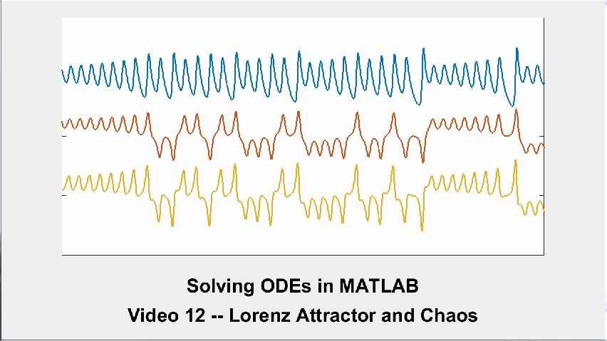
Capture the values t and y and then plot the solution. I'm going to do a plot with the three components offset from each other. And here's an internal function Lorenz equation that is called by ODE 23. And it continuously, every time it called, it modifies the matrix A updates it with the new values of y2.
So let's run that function. And here's the output. Here is the three components of the Lorenz attractor. Time series is functions of t. It's pretty hard to see what's going on here except to say they start out with their initial values, oscillate around them, close them through for a little while, and then begin to deviate.
And it's hard to see what they're doing. They're just oscillating in an unpredictable fashion. We need another graphic to see what's really going on here. I want to write a program called Lorenz GUI. Lorenz Graphic User Interface. That's out of my old book called this one is really out of Numerical Computing with MATLAB, NCM.
OK, I hit the Start button. Here are the two critical points in green. We started near the critical point. We oscillate around the critical point. And here is the orbit. This is just going back and forth. It oscillates around one critical point then decides to go over and oscillate around the other for a while.
It continues around like this forever. This is not periodic. It never repeats. Now, the butterfly is associated with Lorenz in two ways. One is the butterfly effect on the weather. Also, this plot looks like a butterfly. I can grab this with my mouse and rotate it in three dimensions.
So I can get different views of the orbit. It's still being computed. We're adding more and more to the plot. And I can look at it from different points of view to get some notion of how this is proceeding in three dimensions. It almost lives in two dimensions, but not quite.
Earlier, we've seen solutions, differential equations with periodic solutions. Here, this isn't periodic. Just going like this forever. Now, this is perfectly-- this isn't random. This is completely determined by the initial conditions.
If I were to start it over again with those exact conditions, with those exact initial conditions, I'd get exactly this behavior. But it's unpredictable. It's hard to say where this is going. I can clear this out and see the orbit continue to develop. Press Stop.
Now I have a choice. This pull down menu here allows me to choose other values of rho. 28 is the value of rho that is almost always studied, but there's a book by a Colin Sparrow that I've referenced in my in my blog about periodic solutions to Lorenz equations.
And let's take another value. Let me choose rho equal to 160 and clear and restart. Now, after an initial transient, this is now periodic. So this is not chaos. This is a periodic solution.
And these other values of rho, not rho equals 28, that's chaotic, but these other values of rho give periodic solutions with different character. That's a long, interesting story that I talk about in my blog following the work of Sparrow.
Download Code and Files
Related Products
Learn More

Featured Product
MATLAB


Website auswählen
Wählen Sie eine Website aus, um übersetzte Inhalte (sofern verfügbar) sowie lokale Veranstaltungen und Angebote anzuzeigen. Auf der Grundlage Ihres Standorts empfehlen wir Ihnen die folgende Auswahl: United States.
Sie können auch eine Website aus der folgenden Liste auswählen:
Amerika
- América Latina (Español)
- Canada (English)
- United States (English)
Europa
- Belgium (English)
- Denmark (English)
- Deutschland (Deutsch)
- España (Español)
- Finland (English)
- France (Français)
- Ireland (English)
- Italia (Italiano)
- Luxembourg (English)
- Netherlands (English)
- Norway (English)
- Österreich (Deutsch)
- Portugal (English)
- Sweden (English)
- Switzerland
- United Kingdom (English)