tf2ss
Convert transfer function filter parameters to state-space form
Syntax
Description
Examples
Consider the system described by the transfer function
Convert it to state-space form using tf2ss.
b = [0 2 3; 1 2 1];
a = [1 0.4 1];
[A,B,C,D] = tf2ss(b,a)
A = 2×2

   -0.4000   -1.0000
    1.0000         0
B = 2×1

     1
     0
C = 2×2

    2.0000    3.0000
    1.6000         0
D = 2×1

     0
     1
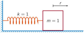
A one-dimensional discrete-time oscillating system consists of a unit mass, , attached to a wall by a spring of unit elastic constant. A sensor samples the acceleration, , of the mass at Hz.

Generate 50 time samples. Define the sampling interval .
Fs = 5;
dt = 1/Fs;
N = 50;
t = dt*(0:N-1);
u = [1 zeros(1,N-1)];
The transfer function of the system has an analytic expression:
.
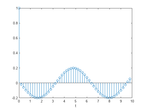
The system is excited with a unit impulse in the positive direction. Compute the time evolution of the system using the transfer function. Plot the response.
bf = [1 -(1+cos(dt)) cos(dt)];
af = [1 -2*cos(dt) 1];
yf = filter(bf,af,u);

stem(t,yf,"o")
xlabel("t")

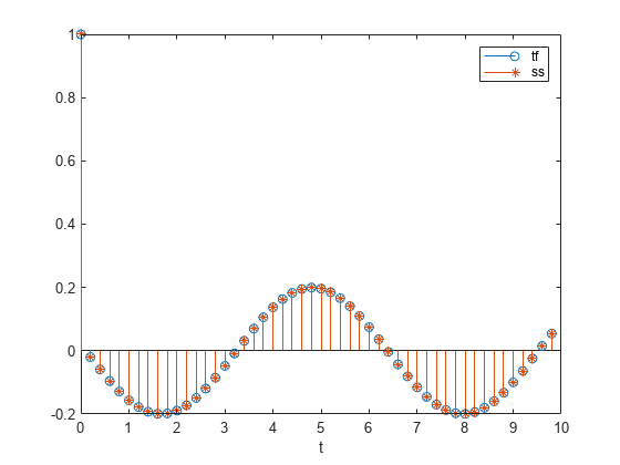
Find the state-space representation of the system. Compute the time evolution starting from an all-zero initial state. Compare it to the transfer function prediction.
[A,B,C,D] = tf2ss(bf,af);

x = [0;0];
for k = 1:N
    y(k) = C*x + D*u(k);
    x = A*x + B*u(k);
end

hold on
stem(t,y,"*")
hold off
legend("tf","ss")

Input Arguments
Transfer function numerator coefficients, specified as a vector or matrix. If
b is a matrix, then each row of b
corresponds to an output of the system.
For discrete-time systems,
bcontains the coefficients in descending powers of z.For continuous-time systems,
bcontains the coefficients in descending powers of s.
For discrete-time systems, b must have a number of columns equal
to the length of a. If the numbers differ, make them equal by padding
zeros. You can use the function eqtflength to accomplish this.
Transfer function denominator coefficients, specified as a vector.
For discrete-time systems,
acontains the coefficients in descending powers of z.For continuous-time systems,
acontains the coefficients in descending powers of s.
Output Arguments
State matrix, returned as a matrix. If the system is described by
n state variables, then A is
n-by-n.
Data Types: single | double
Input-to-state matrix, returned as a matrix. If the system is described by
n state variables, then B is
n-by-1.
Data Types: single | double
State-to-output matrix, returned as a matrix. If the system has q
outputs and is described by n state variables, then
C is q-by-n.
Data Types: single | double
Feedthrough matrix, returned as a matrix. If the system has q
outputs, then D is q-by-1.
Data Types: single | double
More About
tf2ss converts the parameters of a transfer
function representation of a given system to those of an equivalent state-space
representation.
For discrete-time systems, the state-space matrices relate the state vector x, the input u, and the output y:
The transfer function is the Z-transform of the system’s impulse response. It can be expressed in terms of the state-space matrices as
For continuous-time systems, the state-space matrices relate the state vector x, the input u, and the output y:
The transfer function is the Laplace transform of the system’s impulse response. It can be expressed in terms of the state-space matrices as
Extended Capabilities
C/C++ Code Generation
Generate C and C++ code using MATLAB® Coder™.
GPU Code Generation
Generate CUDA® code for NVIDIA® GPUs using GPU Coder™.
Version History
Introduced before R2006a
MATLAB Command
You clicked a link that corresponds to this MATLAB command:
Run the command by entering it in the MATLAB Command Window. Web browsers do not support MATLAB commands.
Select a Web Site
Choose a web site to get translated content where available and see local events and offers. Based on your location, we recommend that you select: .
You can also select a web site from the following list
How to Get Best Site Performance
Select the China site (in Chinese or English) for best site performance. Other MathWorks country sites are not optimized for visits from your location.
Americas
- América Latina (Español)
- Canada (English)
- United States (English)
Europe
- Belgium (English)
- Denmark (English)
- Deutschland (Deutsch)
- España (Español)
- Finland (English)
- France (Français)
- Ireland (English)
- Italia (Italiano)
- Luxembourg (English)
- Netherlands (English)
- Norway (English)
- Österreich (Deutsch)
- Portugal (English)
- Sweden (English)
- Switzerland
- United Kingdom (English)