Latest Contributions
Happy Pi Day!
3.14 π Day has arrived, and this post provides some very cool pi implementations and complete MATLAB code.
Firstly, in order to obtain the first n decimal places of pi, we need to write the following code (to prevent inaccuracies, we need to take a few more tails and perform another operation of taking the first n decimal places when needed):
function Pi=getPi(n)
if nargin<1,n=3;end
Pi=char(vpa(sym(pi),n+10));
Pi=abs(Pi)-48;
Pi=Pi(3:n+2);
end
With this function to obtain the decimal places of pi, our visualization journey has begun~Step by step, from simple to complex~(Please try to use newer versions of MATLAB to run, at least R17b)
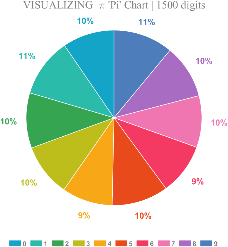
1 Pie chart
Just calculate the proportion of each digit to the first 1500 decimal places:
% 获取pi前1500位小数
Pi=getPi(1500);
% 统计各个数字出现次数
numNum=find([diff(sort(Pi)),1]);
numNum=[numNum(1),diff(numNum)];
% 配色列表
CM=[20,164,199;43,187,170;53,165,81;189,190,28;248,167,22;
232,74,27;244,57,99;240,118,177;168,109,195;78,125,187]./255;
% 绘图并修饰
pieHdl=pie(numNum);
set(gcf,'Color',[1,1,1],'Position',[200,100,620,620]);
for i=1:2:20
pieHdl(i).EdgeColor=[1,1,1];
pieHdl(i).LineWidth=1;
pieHdl(i).FaceColor=CM((i+1)/2,:);
end
for i=2:2:20
pieHdl(i).Color=CM(i/2,:);
pieHdl(i).FontWeight='bold';
pieHdl(i).FontSize=14;
end
% 绘制图例并修饰
lgdHdl=legend(num2cell('0123456789'));
lgdHdl.FontWeight='bold';
lgdHdl.FontSize=11;
lgdHdl.TextColor=[.5,.5,.5];
lgdHdl.Location='southoutside';
lgdHdl.Box='off';
lgdHdl.NumColumns=10;
lgdHdl.ItemTokenSize=[20,15];
title("VISUALIZING \pi 'Pi' Chart | 1500 digits",'FontSize',18,...
'FontName','Times New Roman','Color',[.5,.5,.5])
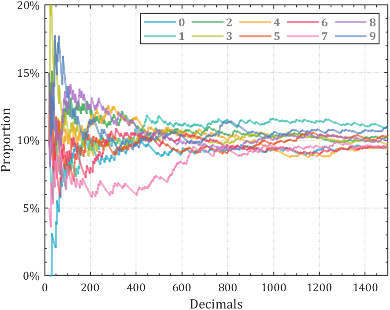
2 line chart
Calculate the change in the proportion of each number:
% 获取pi前1500位小数
Pi=getPi(1500);
% 计算比例变化
Ratio=cumsum(Pi==(0:9)',2);
Ratio=Ratio./sum(Ratio);
D=1:length(Ratio);
% 配色列表
CM=[20,164,199;43,187,170;53,165,81;189,190,28;248,167,22;
232,74,27;244,57,99;240,118,177;168,109,195;78,125,187]./255;
hold on
% 循环绘图
for i=1:10
plot(D(20:end),Ratio(i,20:end),'Color',[CM(i,:),.6],'LineWidth',1.8)
end
% 坐标区域修饰
ax=gca;box on;grid on
ax.YLim=[0,.2];
ax.YTick=0:.05:.2;
ax.XTick=0:200:1400;
ax.YTickLabel={'0%','5%','10%','15%','20%'};
ax.XMinorTick='on';
ax.YMinorTick='on';
ax.LineWidth=.8;
ax.GridLineStyle='-.';
ax.FontName='Cambria';
ax.FontSize=11;
ax.XLabel.String='Decimals';
ax.YLabel.String='Proportion';
ax.XLabel.FontSize=13;
ax.YLabel.FontSize=13;
% 绘制图例并修饰
lgdHdl=legend(num2cell('0123456789'));
lgdHdl.NumColumns=5;
lgdHdl.FontWeight='bold';
lgdHdl.FontSize=11;
lgdHdl.TextColor=[.5,.5,.5];
3 stacked area diagram
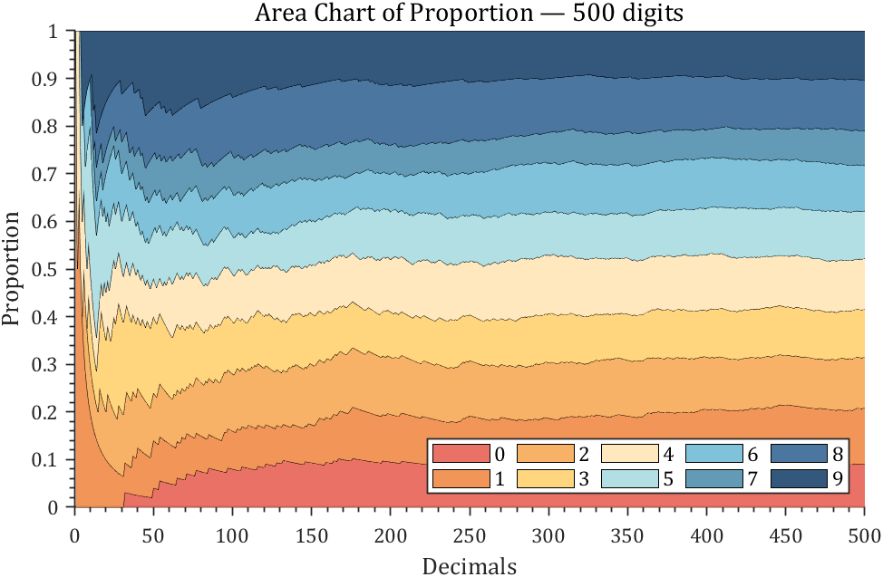
% 获取pi前500位小数
Pi=getPi(500);
% 计算比例变化
Ratio=cumsum(Pi==(0:9)',2);
Ratio=Ratio./sum(Ratio);
% 配色列表
CM=[231,98,84;239,138,71;247,170,88;255,208,111;255,230,183;
170,220,224;114,188,213;82,143,173;55,103,149;30,70,110]./255;
% 绘制堆叠面积图
hold on
areaHdl=area(Ratio');
for i=1:10
areaHdl(i).FaceColor=CM(i,:);
areaHdl(i).FaceAlpha=.9;
end
% 图窗和坐标区域修饰
set(gcf,'Position',[200,100,720,420]);
ax=gca;
ax.YLim=[0,1];
ax.XMinorTick='on';
ax.YMinorTick='on';
ax.LineWidth=.8;
ax.FontName='Cambria';
ax.FontSize=11;
ax.TickDir='out';
ax.XLabel.String='Decimals';
ax.YLabel.String='Proportion';
ax.XLabel.FontSize=13;
ax.YLabel.FontSize=13;
ax.Title.String='Area Chart of Proportion — 500 digits';
ax.Title.FontSize=14;
% 绘制图例并修饰
lgdHdl=legend(num2cell('0123456789'));
lgdHdl.NumColumns=5;
lgdHdl.FontSize=11;
lgdHdl.Location='southeast';
4 connected stacked bar chart
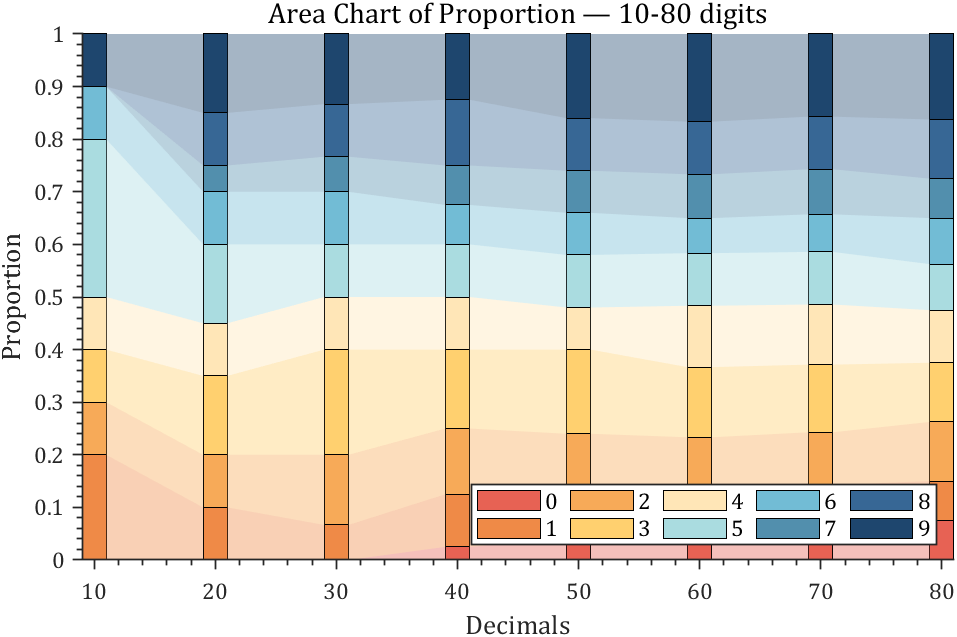
% 获取pi前100位小数
Pi=getPi(100);
% 计算比例变化
Ratio=cumsum(Pi==(0:9)',2);
Ratio=Ratio./sum(Ratio);
X=Ratio(:,10:10:80)';
barHdl=bar(X,'stacked','BarWidth',.2);
CM=[231,98,84;239,138,71;247,170,88;255,208,111;255,230,183;
170,220,224;114,188,213;82,143,173;55,103,149;30,70,110]./255;
for i=1:10
barHdl(i).FaceColor=CM(i,:);
end
% 以下是生成连接的部分
hold on;axis tight
yEndPoints=reshape([barHdl.YEndPoints]',length(barHdl(1).YData),[])';
zeros(1,length(barHdl(1).YData));
yEndPoints=[zeros(1,length(barHdl(1).YData));yEndPoints];
barWidth=barHdl(1).BarWidth;
for i=1:length(barHdl)
for j=1:length(barHdl(1).YData)-1
y1=min(yEndPoints(i,j),yEndPoints(i+1,j));
y2=max(yEndPoints(i,j),yEndPoints(i+1,j));
if y1*y2<0
ty=yEndPoints(find(yEndPoints(i+1,j)*yEndPoints(1:i,j)>=0,1,'last'),j);
y1=min(ty,yEndPoints(i+1,j));
y2=max(ty,yEndPoints(i+1,j));
end
y3=min(yEndPoints(i,j+1),yEndPoints(i+1,j+1));
y4=max(yEndPoints(i,j+1),yEndPoints(i+1,j+1));
if y3*y4<0
ty=yEndPoints(find(yEndPoints(i+1,j+1)*yEndPoints(1:i,j+1)>=0,1,'last'),j+1);
y3=min(ty,yEndPoints(i+1,j+1));
y4=max(ty,yEndPoints(i+1,j+1));
end
fill([j+.5.*barWidth,j+1-.5.*barWidth,j+1-.5.*barWidth,j+.5.*barWidth],...
[y1,y3,y4,y2],barHdl(i).FaceColor,'FaceAlpha',.4,'EdgeColor','none');
end
end
% 图窗和坐标区域修饰
set(gcf,'Position',[200,100,720,420]);
ax=gca;box off
ax.YLim=[0,1];
ax.XMinorTick='on';
ax.YMinorTick='on';
ax.LineWidth=.8;
ax.FontName='Cambria';
ax.FontSize=11;
ax.TickDir='out';
ax.XTickLabel={'10','20','30','40','50','60','70','80'};
ax.XLabel.String='Decimals';
ax.YLabel.String='Proportion';
ax.XLabel.FontSize=13;
ax.YLabel.FontSize=13;
ax.Title.String='Area Chart of Proportion — 10-80 digits';
ax.Title.FontSize=14;
% 绘制图例并修饰
lgdHdl=legend(barHdl,num2cell('0123456789'));
lgdHdl.NumColumns=5;
lgdHdl.FontSize=11;
lgdHdl.Location='southeast';
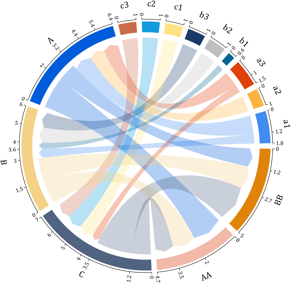
5 bichord chart
Need to use this tool:

% 构建连接矩阵
dataMat=zeros(10,10);
Pi=getPi(1001);
for i=1:1000
dataMat(Pi(i)+1,Pi(i+1)+1)=dataMat(Pi(i)+1,Pi(i+1)+1)+1;
end
BCC=biChordChart(dataMat,'Arrow','on','Label',num2cell('0123456789'));
BCC=BCC.draw();
% 添加刻度
BCC.tickState('on')
% 修改字体,字号及颜色
BCC.setFont('FontName','Cambria','FontSize',17)
set(gcf,'Position',[200,100,820,820]);
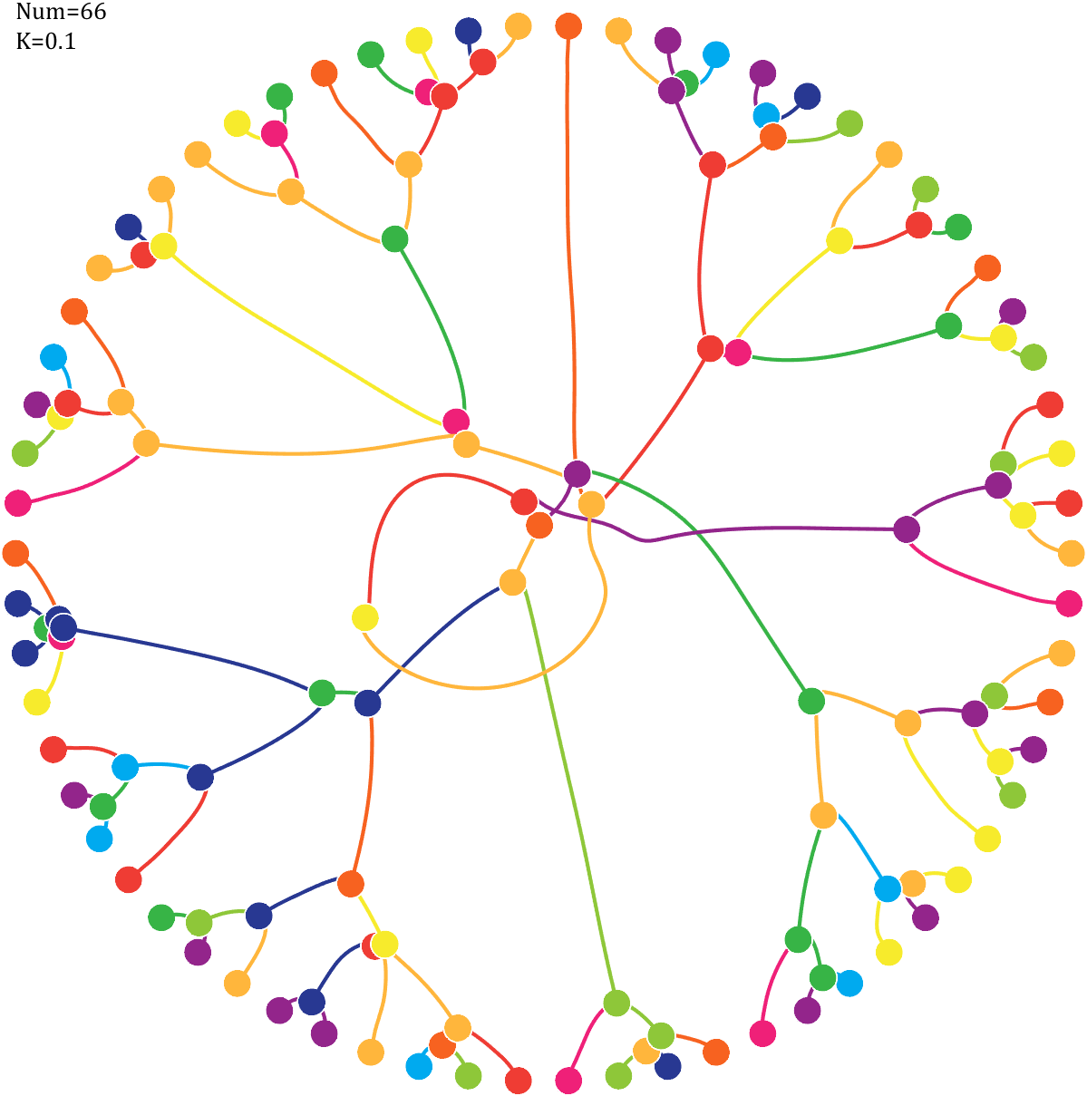
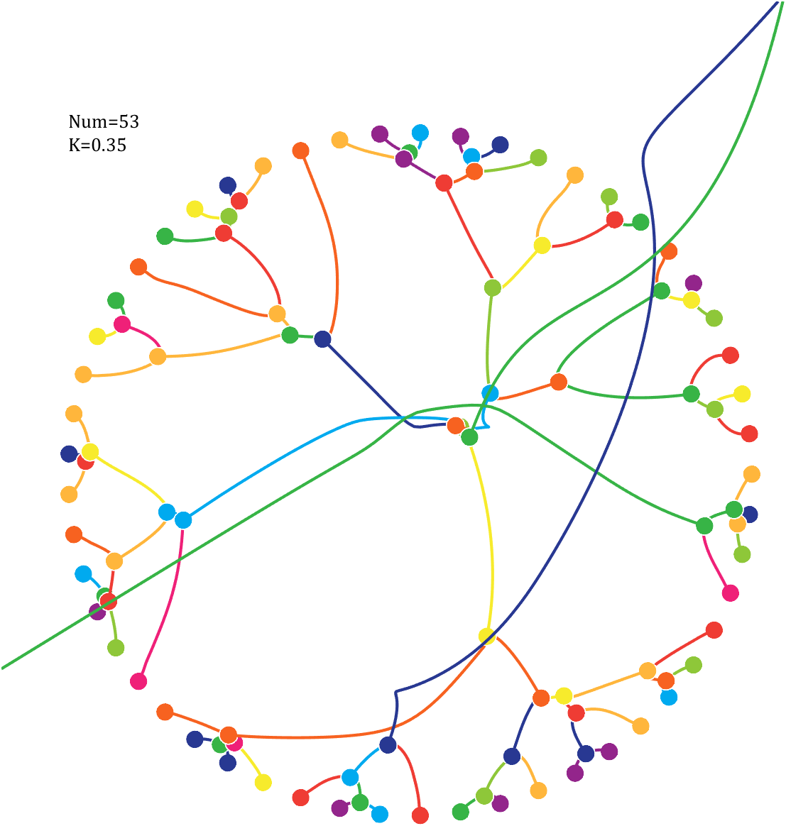
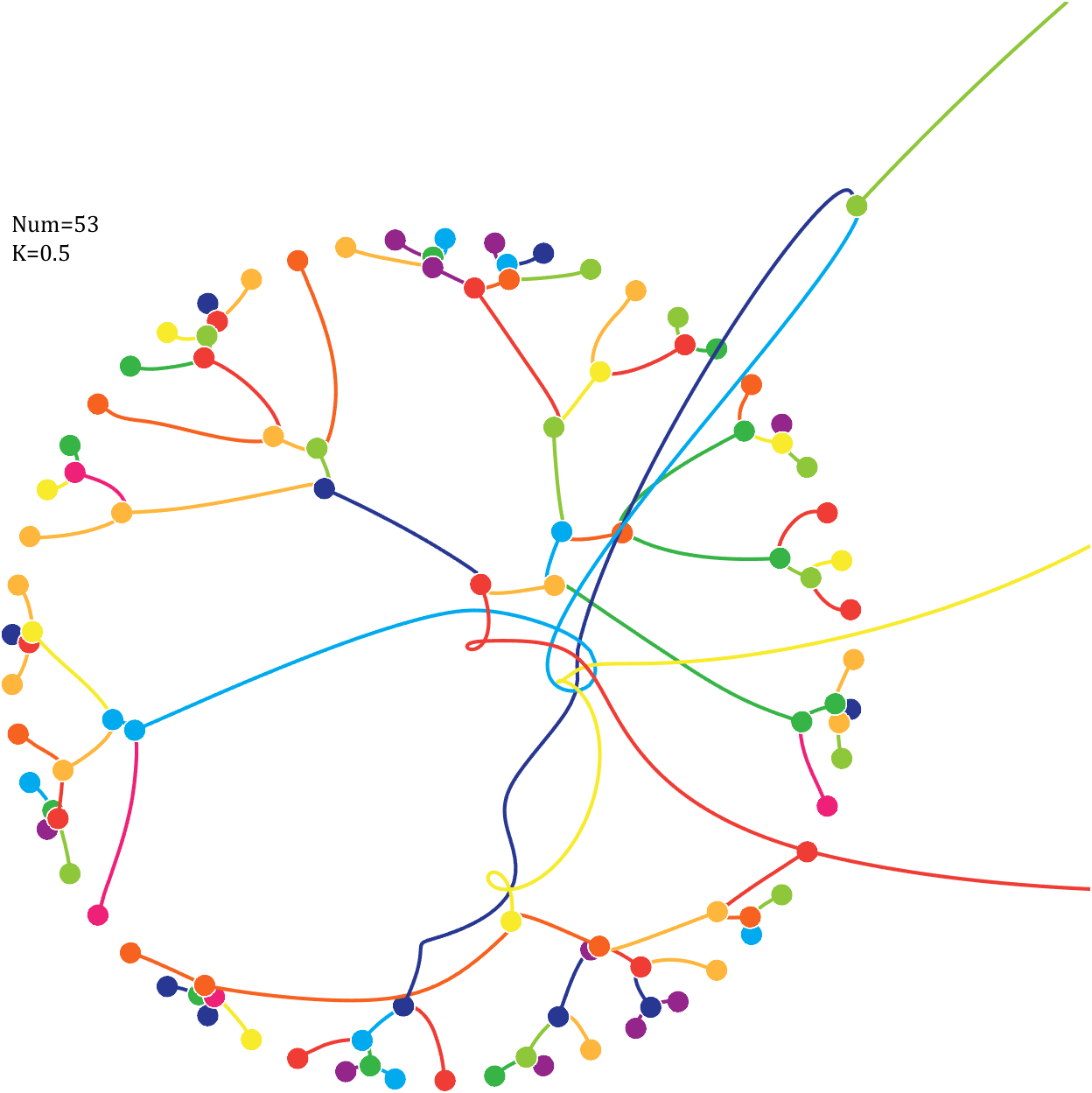
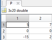
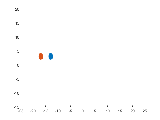
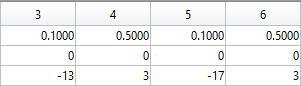
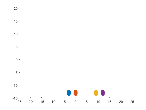
6 Gravity simulation diagram
Imagine each decimal as a small ball with a mass of
For example, if , the weight of ball 0 is 1, ball 9 is 1.2589, the initial velocity of the ball is 0, and it is attracted by other balls. Gravity follows the inverse square law, and if the balls are close enough, they will collide and their value will become
After adding, take the mod, add the velocity direction proportionally, and recalculate the weight.
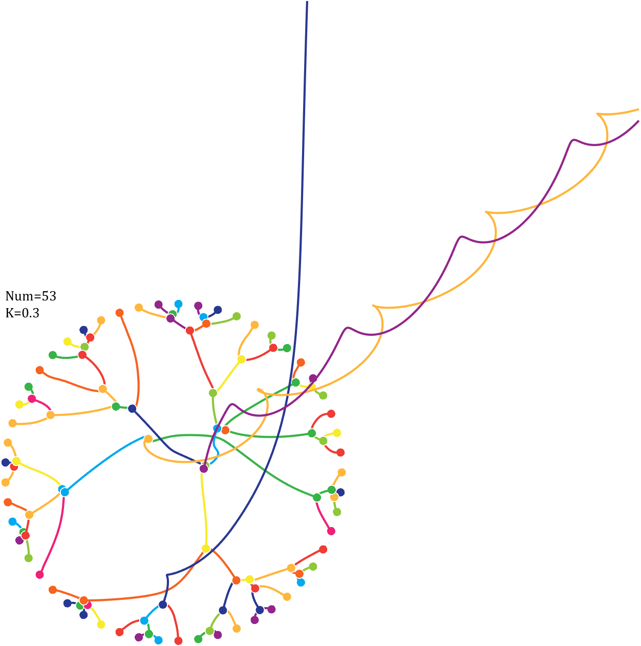
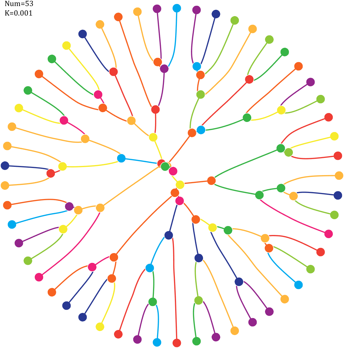
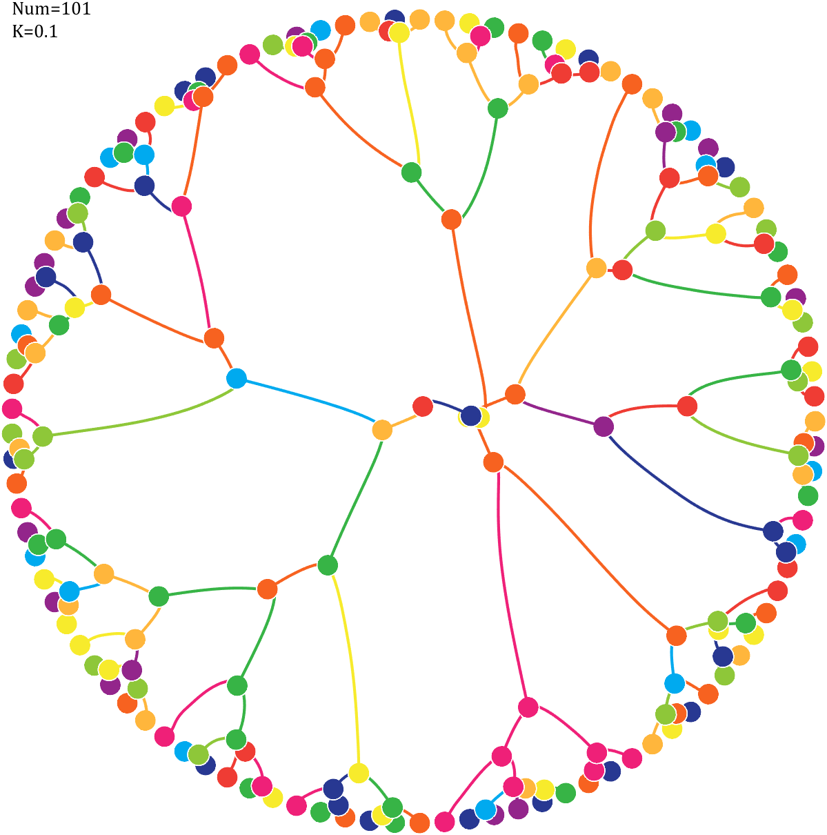
Pi=[3,getPi(71)];K=.18;
% 基础配置
CM=[239,32,120;239,60,52;247,98,32;255,182,60;247,235,44;
142,199,57;55,180,70;0,170,239;40,56,146;147,37,139]./255;
T=linspace(0,2*pi,length(Pi)+1)';
T=T(1:end-1);
ct=linspace(0,2*pi,100);
cx=cos(ct).*.027;
cy=sin(ct).*.027;
% 初始数据
Pi=Pi(:);
N=Pi;
X=cos(T);Y=sin(T);
VX=T.*0;VY=T.*0;
PX=X;PY=Y;
% 未碰撞时初始质量
getM=@(x)(x+1).^K;
M=getM(N);
% 绘制初始圆圈
hold on
for i=1:length(N)
fill(cx+X(i),cy+Y(i),CM(N(i)+1,:),'EdgeColor','w','LineWidth',1)
end
for k=1:800
% 计算加速度
Rn2=1./squareform(pdist([X,Y])).^2;
Rn2(eye(length(X))==1)=0;
MRn2=Rn2.*(M');
AX=X'-X;AY=Y'-Y;
normXY=sqrt(AX.^2+AY.^2);
AX=AX./normXY;AX(eye(length(X))==1)=0;
AY=AY./normXY;AY(eye(length(X))==1)=0;
AX=sum(AX.*MRn2,2)./150000;
AY=sum(AY.*MRn2,2)./150000;
% 计算速度及新位置
VX=VX+AX;X=X+VX;PX=[PX,X];
VY=VY+AY;Y=Y+VY;PY=[PY,Y];
% 检测是否有碰撞
R=squareform(pdist([X,Y]));
R(triu(ones(length(X)))==1)=inf;
[row,col]=find(R<=0.04);
if length(X)==1
break;
end
if ~isempty(row)
% 碰撞的点合为一体
XC=(X(row)+X(col))./2;YC=(Y(row)+Y(col))./2;
VXC=(VX(row).*M(row)+VX(col).*M(col))./(M(row)+M(col));
VYC=(VY(row).*M(row)+VY(col).*M(col))./(M(row)+M(col));
PC=nan(length(row),size(PX,2));
NC=mod(N(row)+N(col),10);
% 删除碰撞点并绘图
uniNum=unique([row;col]);
X(uniNum)=[];VX(uniNum)=[];
Y(uniNum)=[];VY(uniNum)=[];
for i=1:length(uniNum)
plot(PX(uniNum(i),:),PY(uniNum(i),:),'LineWidth',2,'Color',CM(N(uniNum(i))+1,:))
end
PX(uniNum,:)=[];PY(uniNum,:)=[];N(uniNum,:)=[];
% 绘制圆形
for i=1:length(XC)
fill(cx+XC(i),cy+YC(i),CM(NC(i)+1,:),'EdgeColor','w','LineWidth',1)
end
% 补充合体点
X=[X;XC];Y=[Y;YC];VX=[VX;VXC];VY=[VY;VYC];
PX=[PX;PC];PY=[PY;PC];N=[N;NC];M=getM(N);
end
end
for i=1:size(PX,1)
plot(PX(i,:),PY(i,:),'LineWidth',2,'Color',CM(N(i)+1,:))
end
text(-1,1,{['Num=',num2str(length(Pi))];['K=',num2str(K)]},'FontSize',13,'FontName','Cambria')
% 图窗及坐标区域修饰
set(gcf,'Position',[200,100,820,820]);
ax=gca;
ax.Position=[0,0,1,1];
ax.DataAspectRatio=[1,1,1];
ax.XLim=[-1.1,1.1];
ax.YLim=[-1.1,1.1];
ax.XTick=[];
ax.YTick=[];
ax.XColor='none';
ax.YColor='none';
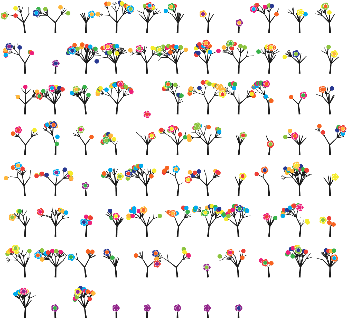
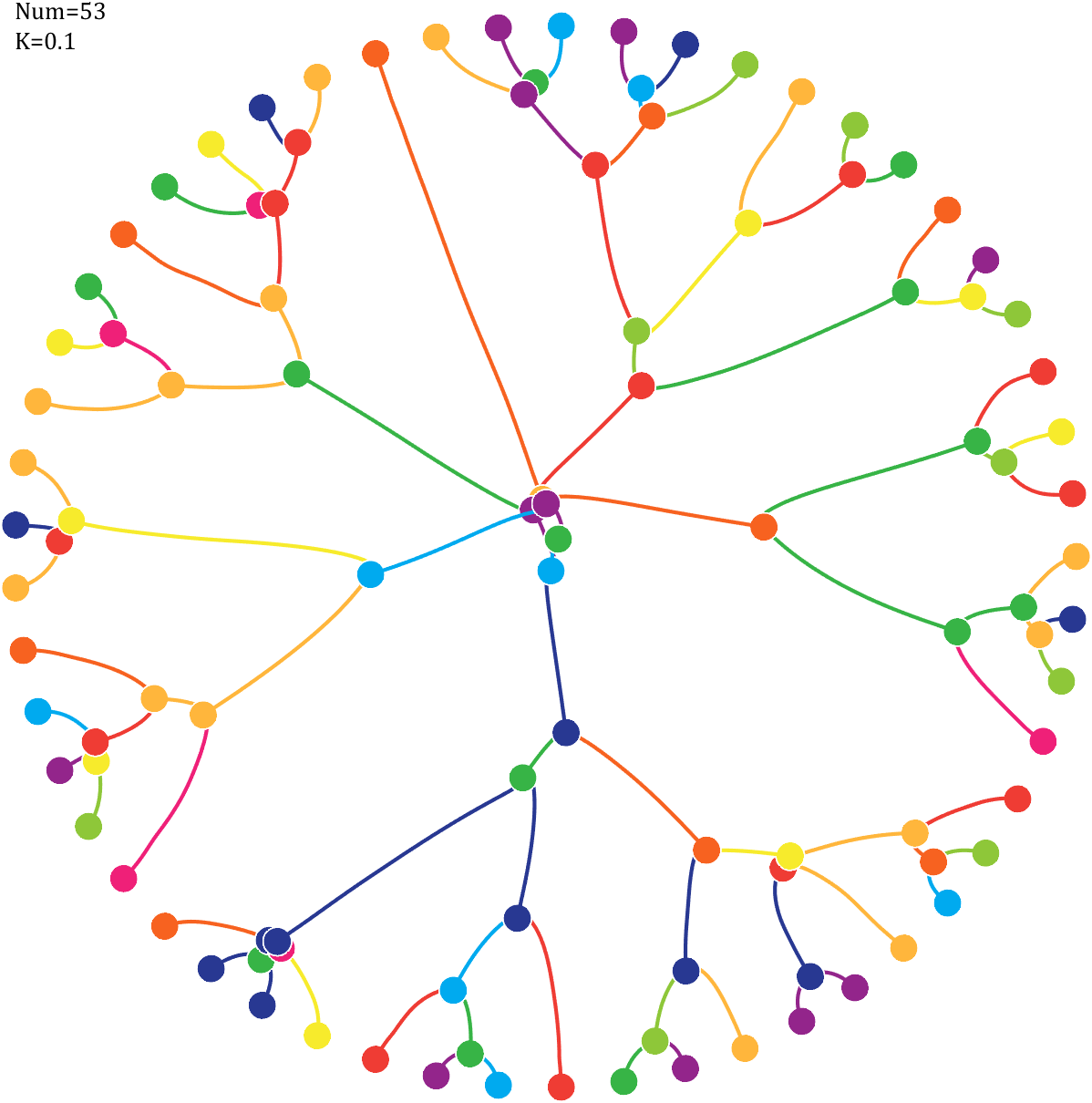
7 forest chart

The method comes from
The digits of π are shown as a forest. Each tree in the forest represents the digits of π up to the next 9. The first 10 trees are "grown" from the digit sets 314159, 2653589, 79, 3238462643383279, 50288419, 7169, 39, 9, 3751058209, and 749.
BRANCHES
The first digit of a tree controls how many branches grow from the trunk of the tree. For example, the first tree's first digit is 3, so you see 3 branches growing from the trunk.
The next digit's branches grow from the end of a branch of the previous digit in left-to-right order. This process continues until all the tree's digits have been used up.
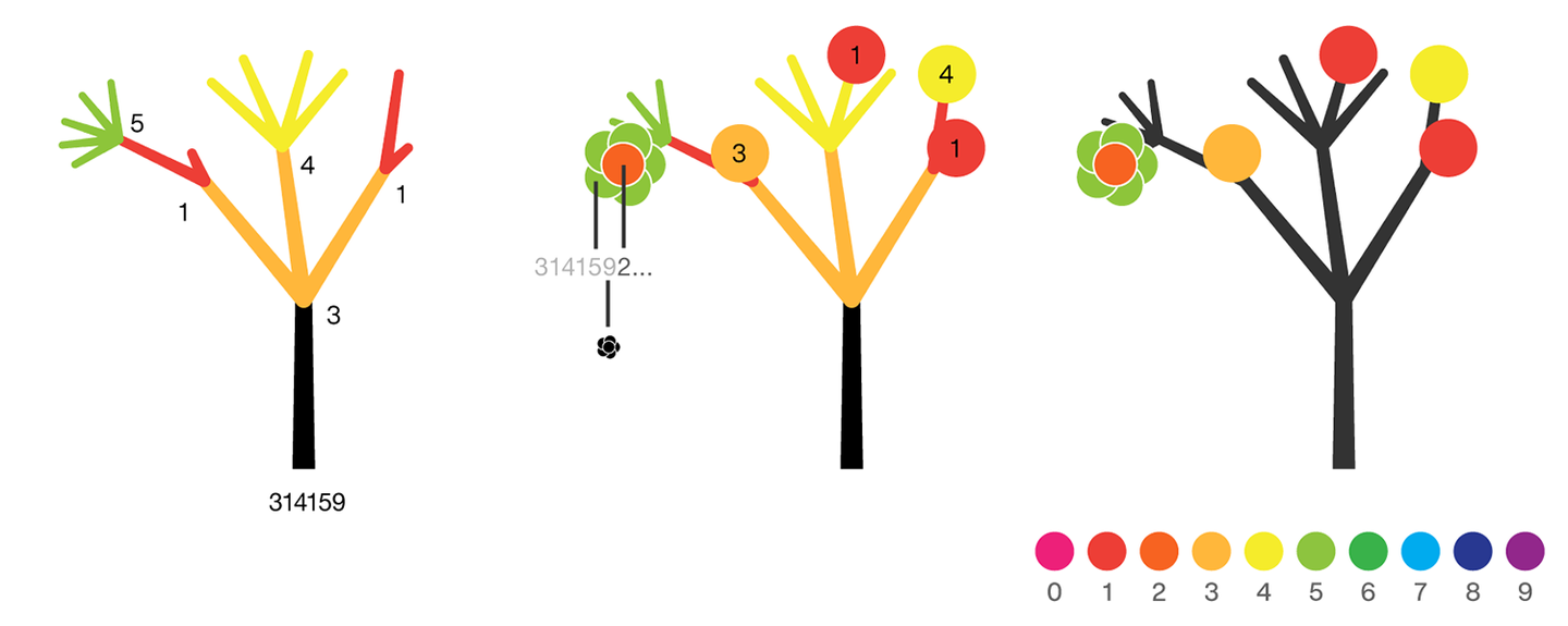
Each tree grows from a set of consecutive digits sampled from the digits of π up to the next 9. The first tree, shown here, grows from 314159. Each of the digits determine how many branches grow at each fork in the tree — the branches here are colored by their corresponding digit to illustrate this. Leaves encode the digits in a left-to-right order. The digit 9 spawns a flower on one of the branches of the previous digit. The branching exception is 0, which terminates the current branch — 0 branches grow!
LEAVES AND FLOWERS
The tree's digits themselves are drawn as circular leaves, color-coded by the digit.
The leaf exception is 9, which causes one of the branches of the previous digit to sprout a flower! The petals of the flower are colored by the digit before the 9 and the center is colored by the digit after the 9, which is on the next tree. This is how the forest propagates.
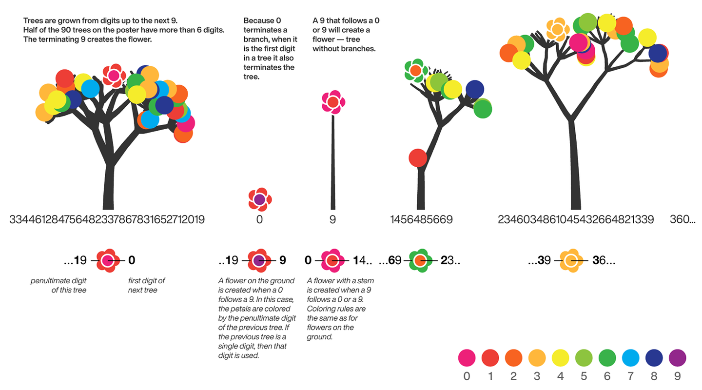
The colors of a flower are determined by the first digit of the next tree and the penultimate digit of the current tree. If the current tree only has one digit, then that digit is used. Leaves are placed at the tips of branches in a left-to-right order — you can "easily" read them off. Additionally, the leaves are distributed within the tree (without disturbing their left-to-right order) to spread them out as much as possible and avoid overlap. This order is deterministic.
The leaf placement exception are the branch set that sprouted the flower. These are not used to grow leaves — the flower needs space!
function PiTree(X,pos,D)
lw=2;
theta=pi/2+(rand(1)-.5).*pi./12;
% 树叶及花朵颜色
CM=[237,32,121;237,62,54;247,99,33;255,183,59;245,236,43;
141,196,63;57,178,74;0,171,238;40,56,145;146,39,139]./255;
hold on
if all(X(1:end-2)==0)
endSet=[pos,pos,theta];
else
kplot(pos(1)+[0,cos(theta)],pos(2)+[0,sin(theta)],lw./.6)
endSet=[pos,pos+[cos(theta),sin(theta)],theta];
% 计算层级
Layer=0;
for i=1:length(X)
Layer=[Layer,ones(1,X(i)).*i];
end
% 计算树枝
if D
for i=1:length(X)-2
if X(i)==0 % 若数值为0则不长树枝
newSet=endSet(1,:);
elseif X(i)==1 % 若数值为1则一长一短两个树枝
tTheta=endSet(1,5);
tTheta=linspace(tTheta+pi/8,tTheta-pi/8,2)'+(rand([2,1])-.5).*pi./8;
newSet=repmat(endSet(1,3:4),[X(i),1]);
newSet=[newSet.*[1;1],newSet+[cos(tTheta),sin(tTheta)].*.7^Layer(i).*[1;.1],tTheta];
else % 其他情况数值为几长几个树枝
tTheta=endSet(1,5);
tTheta=linspace(tTheta+pi/5,tTheta-pi/5,X(i))'+(rand([X(i),1])-.5).*pi./8;
newSet=repmat(endSet(1,3:4),[X(i),1]);
newSet=[newSet,newSet+[cos(tTheta),sin(tTheta)].*.7^Layer(i),tTheta];
end
% 绘制树枝
for j=1:size(newSet,1)
kplot(newSet(j,[1,3]),newSet(j,[2,4]),lw.*.6^Layer(i))
end
endSet=[endSet;newSet];
endSet(1,:)=[];
end
end
end
% 计算叶子和花朵位置
FLSet=endSet(:,3:4);
[~,FLInd]=sort(FLSet(:,1));
FLSet=FLSet(FLInd,:);
[~,tempInd]=sort(rand([1,size(FLSet,1)]));
tempInd=sort(tempInd(1:length(X)-2));
flowerInd=tempInd(randi([1,length(X)-2],[1,1]));
leafInd=tempInd(tempInd~=flowerInd);
% 绘制树叶
for i=1:length(leafInd)
scatter(FLSet(leafInd(i),1),FLSet(leafInd(i),2),70,'filled','CData',CM(X(i)+1,:))
end
% 绘制花朵
for i=1:5
% if ~D
% tC=CM(X(end)+1,:);
% else
% tC=CM(X(end-2)+1,:);
% end
scatter(FLSet(flowerInd,1)+cos(pi*2*i/5).*.18,FLSet(flowerInd,2)+sin(pi*2*i/5).*.18,60,...
'filled','CData',CM(X(end-2)+1,:),'MarkerEdgeColor',[1,1,1])
end
scatter(FLSet(flowerInd,1),FLSet(flowerInd,2),60,'filled','CData',CM(X(end)+1,:),'MarkerEdgeColor',[1,1,1])
drawnow;%axis tight
% =========================================================================
function kplot(XX,YY,LW,varargin)
LW=linspace(LW,LW*.6,10);%+rand(1,20).*LW./10;
XX=linspace(XX(1),XX(2),11)';
XX=[XX(1:end-1),XX(2:end)];
YY=linspace(YY(1),YY(2),11)';
YY=[YY(1:end-1),YY(2:end)];
for ii=1:10
plot(XX(ii,:),YY(ii,:),'LineWidth',LW(ii),'Color',[.1,.1,.1])
end
end
end
main part:
Pi=[3,getPi(800)];
pos9=[0,find(Pi==9)];
set(gcf,'Position',[200,50,900,900],'Color',[1,1,1]);
ax=gca;hold on
ax.Position=[0,0,1,1];
ax.DataAspectRatio=[1,1,1];
ax.XLim=[.5,36];
ax.XTick=[];
ax.YTick=[];
ax.XColor='none';
ax.YColor='none';
for j=1:8
for i=1:11
n=i+(j-1)*11;
if n<=85
tPi=Pi((pos9(n)+1):pos9(n+1)+1);
if length(tPi)>2
PiTree(tPi,[0+i*3,0-j*4],true);
else
PiTree([Pi(pos9(n)),tPi],[0+i*3,0-j*4],false);
end
end
end
end
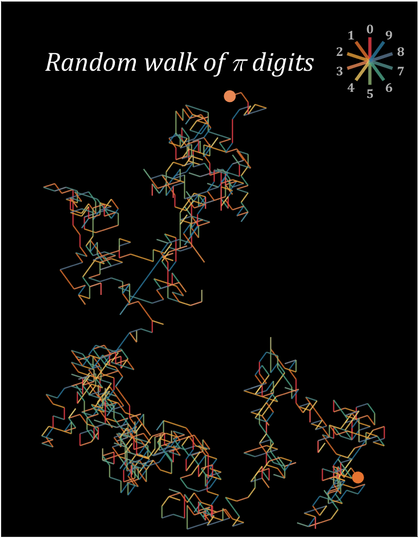
8 random walk
n=1200;
% 获取pi前n位小数
Pi=getPi(n);
CM=[239,65,75;230,115,48;229,158,57;232,136,85;239,199,97;
144,180,116;78,166,136;81,140,136;90,118,142;43,121,159]./255;
hold on
endPoint=[0,0];
t=linspace(0,2*pi,100);
T=linspace(0,2*pi,11)+pi/2;
fill(endPoint(1)+cos(t).*.5,endPoint(2)+sin(t).*.5,CM(Pi(1)+1,:),'EdgeColor','none')
for i=1:n
theta=T(Pi(i)+1);
plot(endPoint(1)+[0,cos(theta)],endPoint(2)+[0,sin(theta)],'Color',[CM(Pi(i)+1,:),.8],'LineWidth',1.2);
endPoint=endPoint+[cos(theta),sin(theta)];
end
fill(endPoint(1)+cos(t).*.5,endPoint(2)+sin(t).*.5,CM(Pi(n)+1,:),'EdgeColor','none')
% 图窗和坐标区域修饰
set(gcf,'Position',[200,100,820,820]);
ax=gca;
ax.XTick=[];
ax.YTick=[];
ax.Color=[0,0,0];
ax.DataAspectRatio=[1,1,1];
ax.XLim=[-30,5];
ax.YLim=[-5,40];
% 绘制图例
endPoint=[1,35];
for i=1:10
theta=T(i);
plot(endPoint(1)+[0,cos(theta).*2],endPoint(2)+[0,sin(theta).*2],'Color',[CM(i,:),.8],'LineWidth',3);
text(endPoint(1)+cos(theta).*2.7,endPoint(2)+sin(theta).*2.7,num2str(i-1),'Color',[1,1,1].*.7,...
'FontSize',12,'FontWeight','bold','FontName','Cambria','HorizontalAlignment','center')
end
text(-15,35,'Random walk of \pi digits','Color',[1,1,1],'FontName','Cambria',...
'HorizontalAlignment','center','FontSize',25,'FontAngle','italic')
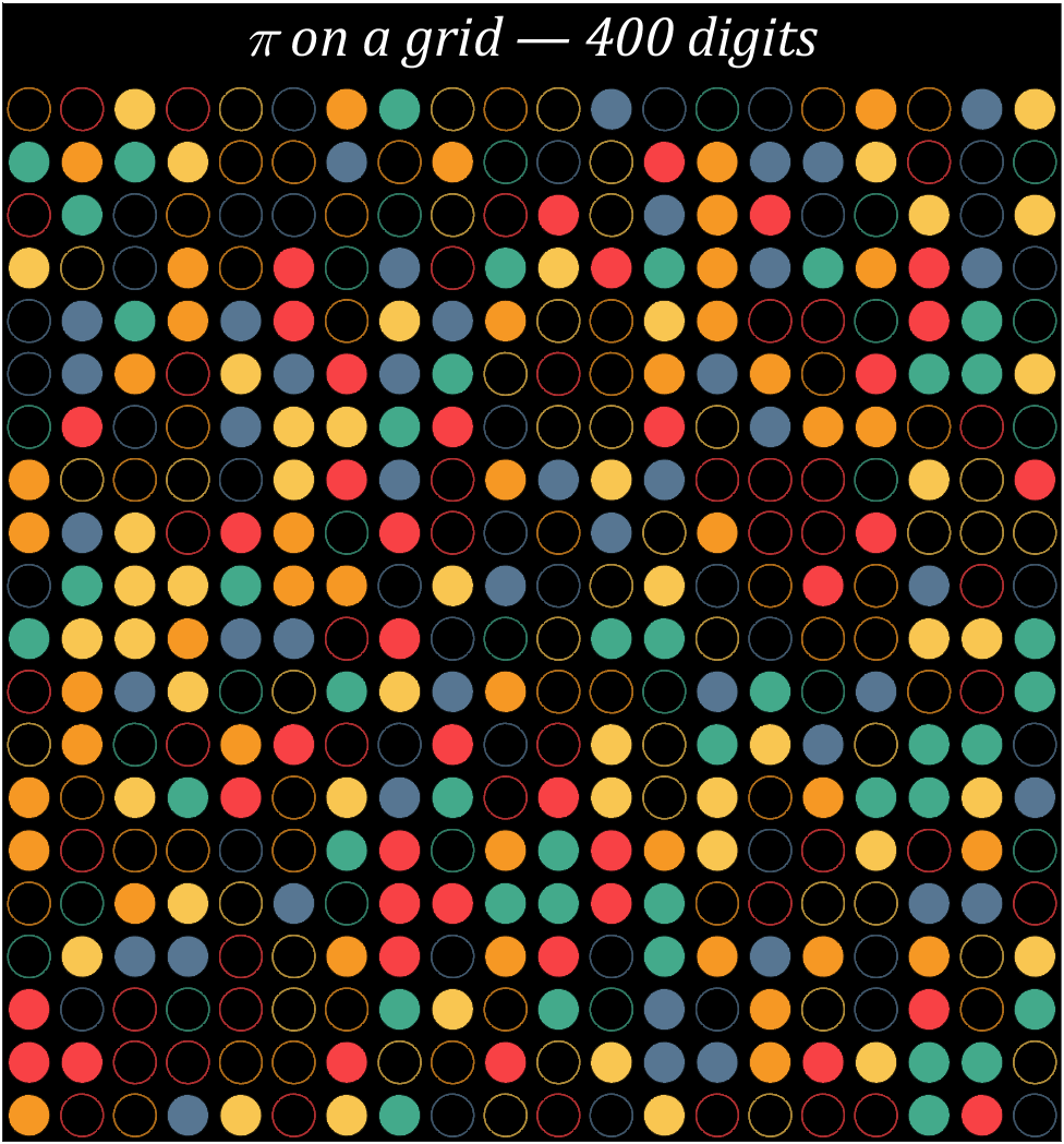
9 grid chart
Pi=[3,getPi(399)];
% 配色数据
CM=[248,65,69;246,152,36;249,198,81;67,170,139;87,118,146]./255;
% 绘制圆圈
hold on
t=linspace(0,2*pi,100);
x=cos(t).*.8.*.5;
y=sin(t).*.8.*.5;
for i=1:400
[col,row]=ind2sub([20,20],i);
if mod(Pi(i),2)==0
fill(x+col,y+row,CM(round((Pi(i)+1)/2),:),'LineWidth',1,'EdgeAlpha',.8)
else
fill(x+col,y+row,[0,0,0],'EdgeColor',CM(round((Pi(i)+1)/2),:),'LineWidth',1,'EdgeAlpha',.7)
end
end
text(10.5,-.4,'\pi on a grid — 400 digits','Color',[1,1,1],'FontName','Cambria',...
'HorizontalAlignment','center','FontSize',25,'FontAngle','italic')
% 图窗和坐标区域修饰
set(gcf,'Position',[200,100,820,820]);
ax=gca;
ax.YDir='reverse';
ax.XLim=[.5,20.5];
ax.YLim=[-1,20.5];
ax.XTick=[];
ax.YTick=[];
ax.Color=[0,0,0];
ax.DataAspectRatio=[1,1,1];
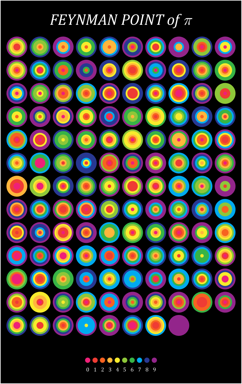
10 scale grid diagram
Let's still put the numbers in the form of circles, but the difference is that six numbers are grouped together, and the pure purple circle at the end is the six 9s that we are familiar with decimal places 762-767
Pi=[3,getPi(767)];
% 762-767
% 配色数据
CM=[239,32,120;239,60,52;247,98,32;255,182,60;247,235,44;
142,199,57;55,180,70;0,170,239;40,56,146;147,37,139]./255;
% 绘制圆圈
hold on
t=linspace(0,2*pi,100);
x=cos(t).*.9.*.5;
y=sin(t).*.9.*.5;
for i=1:6:length(Pi)
n=round((i-1)/6+1);
[col,row]=ind2sub([10,13],n);
tNum=Pi(i:i+5);
numNum=find([diff(sort(tNum)),1]);
numNum=[numNum(1),diff(numNum)];
cumNum=cumsum(numNum);
uniNum=unique(tNum);
for j=length(cumNum):-1:1
fill(x./6.*cumNum(j)+col,y./6.*cumNum(j)+row,CM(uniNum(j)+1,:),'EdgeColor','none')
end
end
% 绘制图例
for i=1:10
fill(x./4+5.5+(i-5.5)*.32,y./4+14.5,CM(i,:),'EdgeColor','none')
text(5.5+(i-5.5)*.32,14.9,num2str(i-1),'Color',[1,1,1],'FontSize',...
9,'FontName','Cambria','HorizontalAlignment','center')
end
text(5.5,-.2,'FEYNMAN POINT of \pi','Color',[1,1,1],'FontName','Cambria',...
'HorizontalAlignment','center','FontSize',25,'FontAngle','italic')
% 图窗和坐标区域修饰
set(gcf,'Position',[200,100,600,820]);
ax=gca;
ax.YDir='reverse';
ax.Position=[0,0,1,1];
ax.XLim=[.3,10.7];
ax.YLim=[-1,15.5];
ax.XTick=[];
ax.YTick=[];
ax.Color=[0,0,0];
ax.DataAspectRatio=[1,1,1];
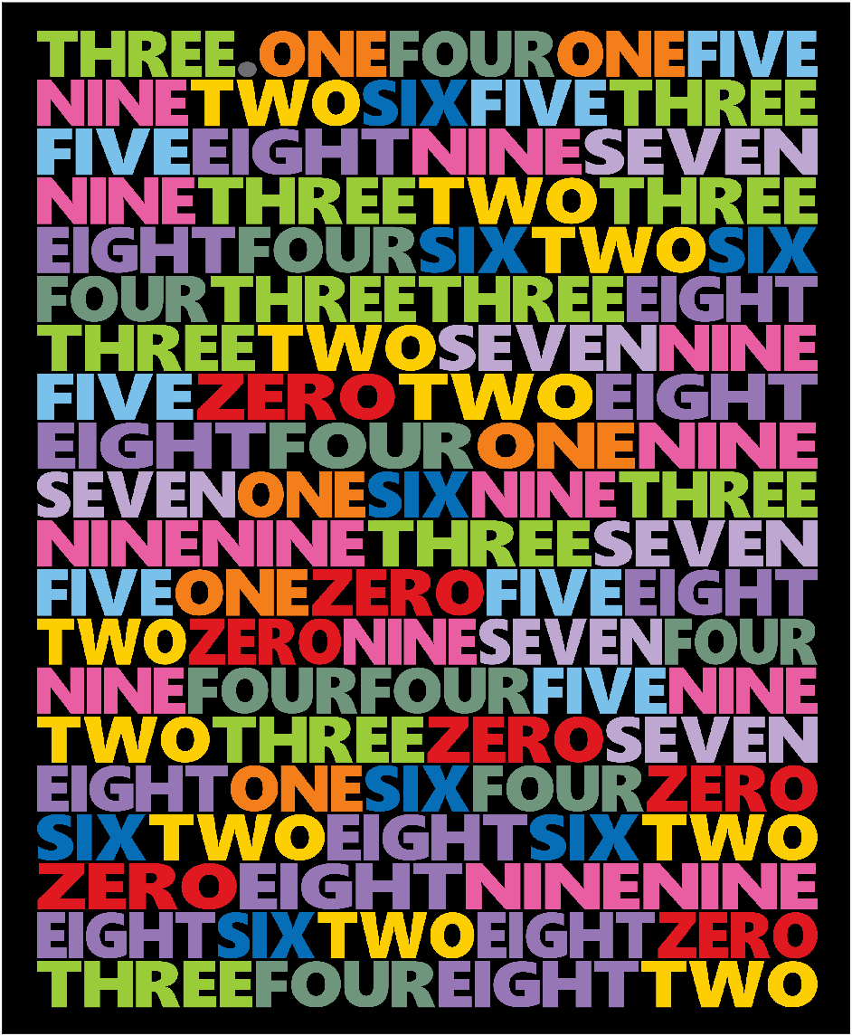
11 text chart

First, write a code to generate an image of each letter:
function getLogo
if ~exist('image','dir')
mkdir('image\')
end
logoSet=['.',char(65:90)];
for i=1:27
figure();
ax=gca;
ax.XLim=[-1,1];
ax.YLim=[-1,1];
ax.XColor='none';
ax.YColor='none';
ax.DataAspectRatio=[1,1,1];
logo=logoSet(i);
hold on
text(0,0,logo,'HorizontalAlignment','center','FontSize',320,'FontName','Segoe UI Black')
exportgraphics(ax,['image\',logo,'.png'])
close
end
dotPic=imread('image\..png');
newDotPic=uint8(ones([400,size(dotPic,2),3]).*255);
newDotPic(end-size(dotPic,1)+1:end,:,1)=dotPic(:,:,1);
newDotPic(end-size(dotPic,1)+1:end,:,2)=dotPic(:,:,2);
newDotPic(end-size(dotPic,1)+1:end,:,3)=dotPic(:,:,3);
imwrite(newDotPic,'image\..png')
S=20;
for i=1:27
logo=logoSet(i);
tPic=imread(['image\',logo,'.png']);
sz=size(tPic,[1,2]);
sz=round(sz./sz(1).*400);
tPic=imresize(tPic,sz);
tBox=uint8(255.*ones(size(tPic,[1,2])+S));
tBox(S+1:S+size(tPic,1),S+1:S+size(tPic,2))=tPic(:,:,1);
imwrite(cat(3,tBox,tBox,tBox),['image\',logo,'.png'])
end
end

Pi=[3,-1,getPi(150)];
CM=[109,110,113;224,25,33;244,126,26;253,207,2;154,203,57;111,150,124;
121,192,235;6,109,183;190,168,209;151,118,181;233,93,163]./255;
ST={'.','ZERO','ONE','TWO','THREE','FOUR','FIVE','SIX','SEVEN','EIGHT','NINE'};
n=1;
hold on
% 循环绘制字母
for i=1:20%:10
STList='';
NMList=[];
PicListR=uint8(zeros(400,0));
PicListG=uint8(zeros(400,0));
PicListB=uint8(zeros(400,0));
% PicListA=uint8(zeros(400,0));
for j=1:6
STList=[STList,ST{Pi(n)+2}];
NMList=[NMList,ones(size(ST{Pi(n)+2})).*(Pi(n)+2)];
n=n+1;
if length(STList)>15&&length(STList)+length(ST{Pi(n)+2})>20
break;
end
end
for k=1:length(STList)
tPic=imread(['image\',STList(k),'.png']);
% PicListA=[PicListA,tPic(:,:,1)];
PicListR=[PicListR,(255-tPic(:,:,1)).*CM(NMList(k),1)];
PicListG=[PicListG,(255-tPic(:,:,2)).*CM(NMList(k),2)];
PicListB=[PicListB,(255-tPic(:,:,3)).*CM(NMList(k),3)];
end
PicList=cat(3,PicListR,PicListG,PicListB);
image([-1200,1200],[0,150]-(i-1)*150,flipud(PicList))
end
% 图窗及坐标区域修饰
set(gcf,'Position',[200,100,600,820]);
ax=gca;
ax.DataAspectRatio=[1,1,1];
ax.XLim=[-1300,1300];
ax.Position=[0,0,1,1];
ax.XTick=[];
ax.YTick=[];
ax.Color=[0,0,0];
ax.YLim=[-19*150-80,230];
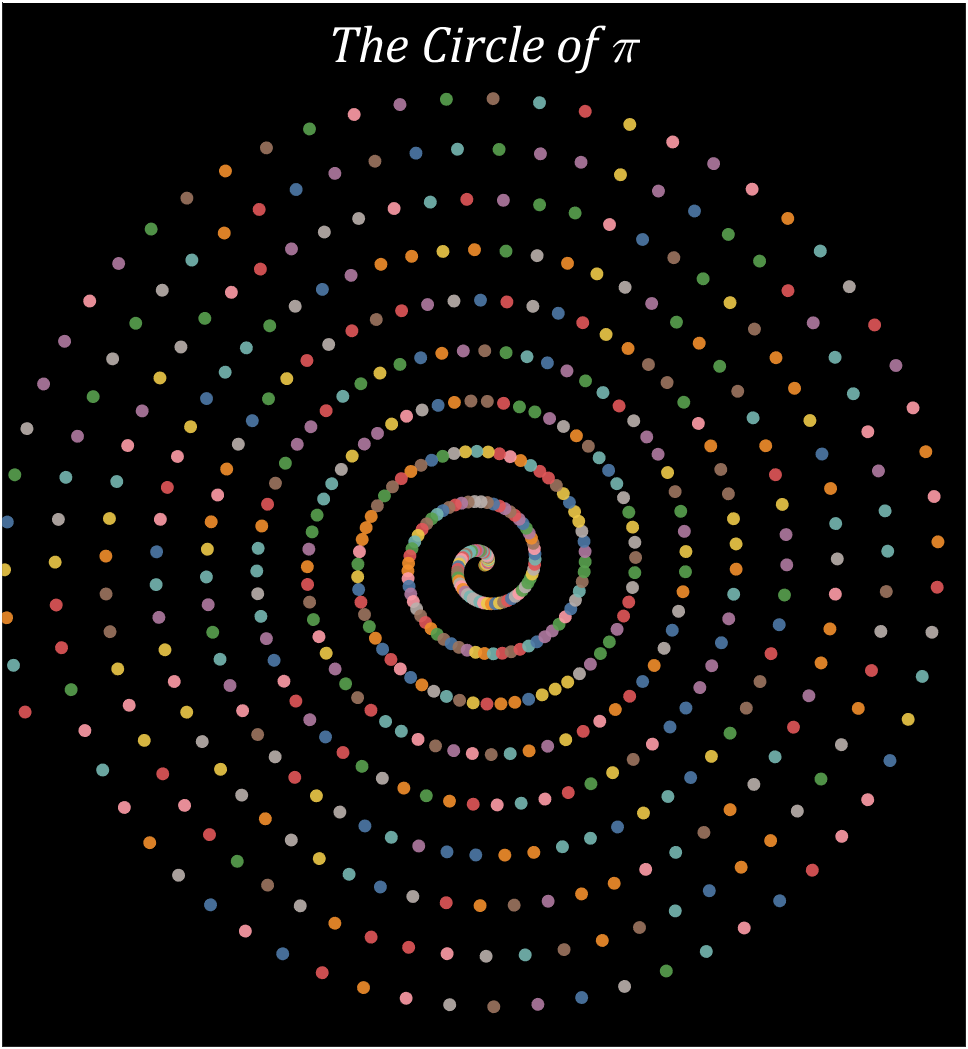
12 spiral chart
Pi=getPi(600);
% 配色列表
CM=[78,121,167;242,142,43;225,87,89;118,183,178;89,161,79;
237,201,72;176,122,161;255,157,167;156,117,95;186,176,172]./255;
% 绘制圆圈
hold on
t=linspace(0,2*pi,100);
x=cos(t).*.8;
y=sin(t).*.8;
for i=1:600
X=i.*cos(i./10)./10;
Y=i.*sin(i./10)./10;
fill(X+x,Y+y,CM(Pi(i)+1,:),'EdgeColor','none','FaceAlpha',.9)
end
text(0,65,'The Circle of \pi','Color',[1,1,1],'FontName','Cambria',...
'HorizontalAlignment','center','FontSize',25,'FontAngle','italic')
% 图窗和坐标区域修饰
set(gcf,'Position',[200,100,820,820]);
ax=gca;
ax.XLim=[-60,60];
ax.YLim=[-60,70];
ax.XTick=[];
ax.YTick=[];
ax.Color=[0,0,0];
ax.DataAspectRatio=[1,1,1];
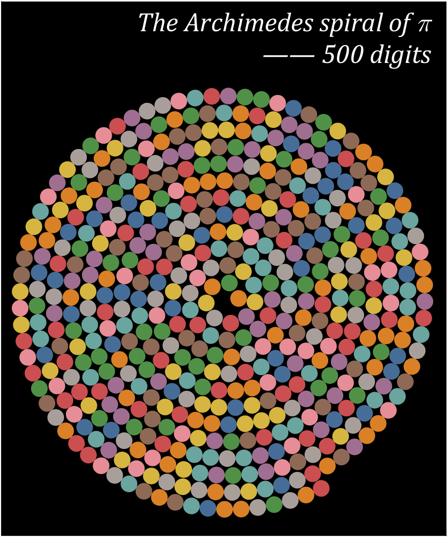
13 Archimedean spiral diagram
a=1;b=.227;
Pi=getPi(500);
% 配色列表
CM=[78,121,167;242,142,43;225,87,89;118,183,178;89,161,79;
237,201,72;176,122,161;255,157,167;156,117,95;186,176,172]./255;
% 绘制圆圈
hold on
T=0;R=1;
t=linspace(0,2*pi,100);
x=cos(t).*.7;
y=sin(t).*.7;
for i=1:500
X=R.*cos(T);Y=R.*sin(T);
fill(X+x,Y+y,CM(Pi(i)+1,:),'EdgeColor','none','FaceAlpha',.9)
T=T+1./R.*1.4;
R=a+b*T;
end
text(17.25,22,{'The Archimedes spiral of \pi';'—— 500 digits'},...
'Color',[1,1,1],'FontName','Cambria',...
'HorizontalAlignment','right','FontSize',25,'FontAngle','italic')
% 图窗和坐标区域修饰
set(gcf,'Position',[200,100,820,820]);
ax=gca;
ax.XLim=[-19,18.5];
ax.YLim=[-20,25];
ax.XTick=[];
ax.YTick=[];
ax.Color=[0,0,0];
ax.DataAspectRatio=[1,1,1];
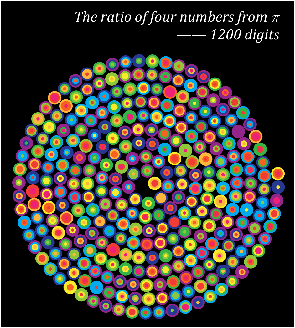
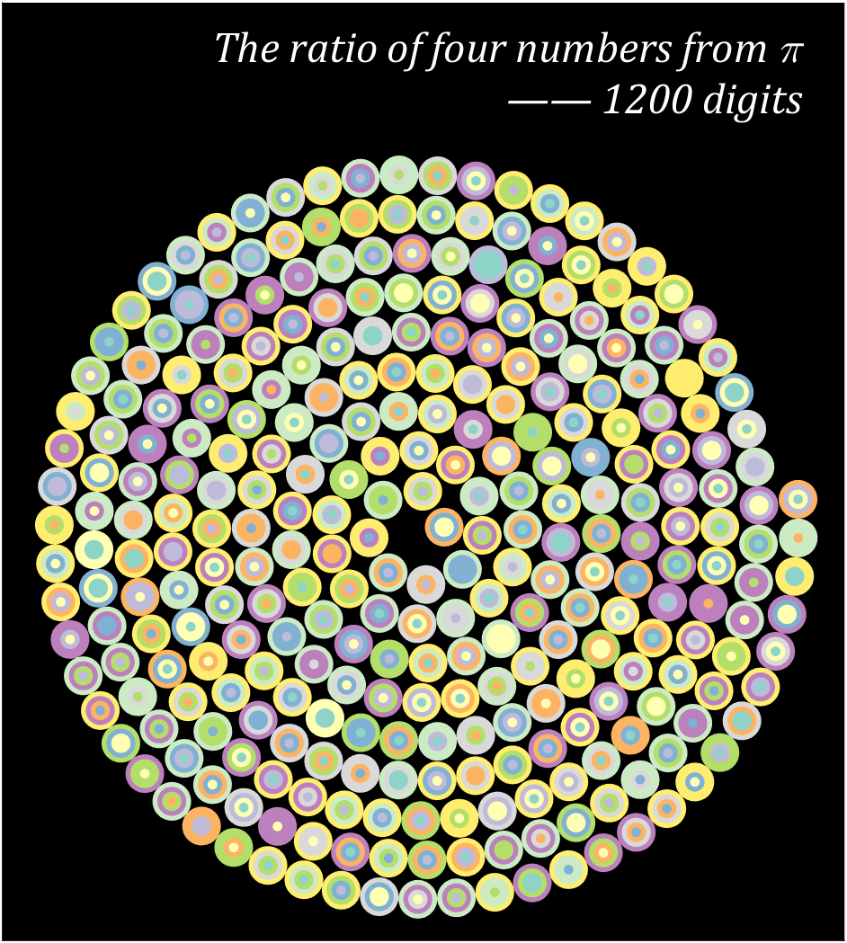
14 proportional Archimedean spiral diagram
Pi=[3,getPi(1199)];
% 配色数据
CM=[239,32,120;239,60,52;247,98,32;255,182,60;247,235,44;
142,199,57;55,180,70;0,170,239;40,56,146;147,37,139]./255;
% CM=slanCM(184,10);
% 绘制圆圈
hold on
T=0;R=1;
t=linspace(0,2*pi,100);
x=cos(t).*.7;
y=sin(t).*.7;
for i=1:4:length(Pi)
X=R.*cos(T);Y=R.*sin(T);
tNum=Pi(i:i+3);
numNum=find([diff(sort(tNum)),1]);
numNum=[numNum(1),diff(numNum)];
cumNum=cumsum(numNum);
uniNum=unique(tNum);
for j=length(cumNum):-1:1
fill(x./4.*cumNum(j)+X,y./4.*cumNum(j)+Y,CM(uniNum(j)+1,:),'EdgeColor','none')
end
T=T+1./R.*1.4;
R=a+b*T;
end
text(14,16.5,{'The ratio of four numbers from \pi';'—— 1200 digits'},...
'Color',[1,1,1],'FontName','Cambria',...
'HorizontalAlignment','right','FontSize',23,'FontAngle','italic')
% 图窗和坐标区域修饰
set(gcf,'Position',[200,100,820,820]);
ax=gca;
ax.XLim=[-15,15.5];
ax.YLim=[-15,19];
ax.XTick=[];
ax.YTick=[];
ax.Color=[0,0,0];
ax.DataAspectRatio=[1,1,1];
15 graph
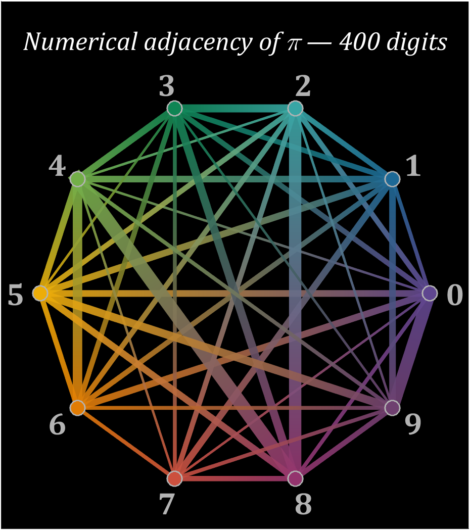
% 构建连接矩阵
corrMat=zeros(10,10);
Pi=getPi(401);
for i=1:400
corrMat(Pi(i)+1,Pi(i+1)+1)=corrMat(Pi(i)+1,Pi(i+1)+1)+1;
end
% 配色列表
colorList=[0.3725 0.2745 0.5647
0.1137 0.4118 0.5882
0.2196 0.6510 0.6471
0.0588 0.5216 0.3294
0.4510 0.6863 0.2824
0.9294 0.6784 0.0314
0.8824 0.4863 0.0196
0.8000 0.3137 0.2431
0.5804 0.2039 0.4314
0.4353 0.2510 0.4392];
t=linspace(0,2*pi,11);t=t(1:10)';
posXY=[cos(t),sin(t)];
maxWidth=max(corrMat(corrMat>0));
minWidth=min(corrMat(corrMat>0));
ttList=linspace(0,1,3)';
% 循环绘图
hold on
for i=1:size(corrMat,1)
for j=i+1:size(corrMat,2)
if corrMat(i,j)>0
tW=(corrMat(i,j)-minWidth)./(maxWidth-minWidth);
colorData=(1-ttList).*colorList(i,:)+ttList.*colorList(j,:);
CData(:,:,1)=colorData(:,1);
CData(:,:,2)=colorData(:,2);
CData(:,:,3)=colorData(:,3);
% 绘制连线
fill(linspace(posXY(i,1),posXY(j,1),3),...
linspace(posXY(i,2),posXY(j,2),3),[0,0,0],'LineWidth',tW.*12+1,...
'CData',CData,'EdgeColor','interp','EdgeAlpha',.7,'FaceAlpha',.7)
end
end
% 绘制圆点
scatter(posXY(i,1),posXY(i,2),200,'filled','LineWidth',1.2,...
'MarkerFaceColor',colorList(i,:),'MarkerEdgeColor',[.7,.7,.7]);
text(posXY(i,1).*1.13,posXY(i,2).*1.13,num2str(i-1),'Color',[1,1,1].*.7,...
'FontSize',30,'FontWeight','bold','FontName','Cambria','HorizontalAlignment','center')
end
text(0,1.3,'Numerical adjacency of \pi — 400 digits','Color',[1,1,1],'FontName','Cambria',...
'HorizontalAlignment','center','FontSize',25,'FontAngle','italic')
% 图窗和坐标区域修饰
set(gcf,'Position',[200,100,820,820]);
ax=gca;
ax.XLim=[-1.2,1.2];
ax.YLim=[-1.21,1.5];
ax.XTick=[];
ax.YTick=[];
ax.Color=[0,0,0];
ax.DataAspectRatio=[1,1,1];
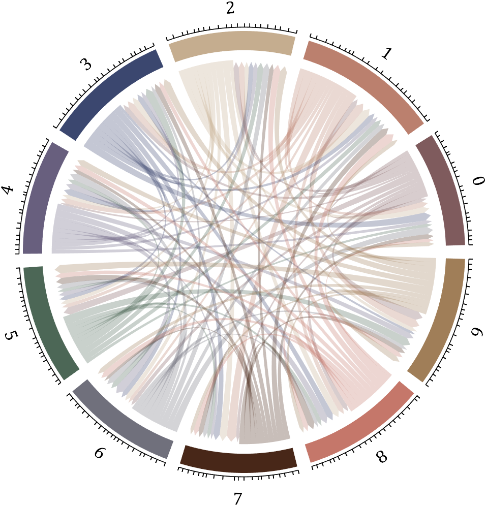
16 circos chart
Need to use this tool:
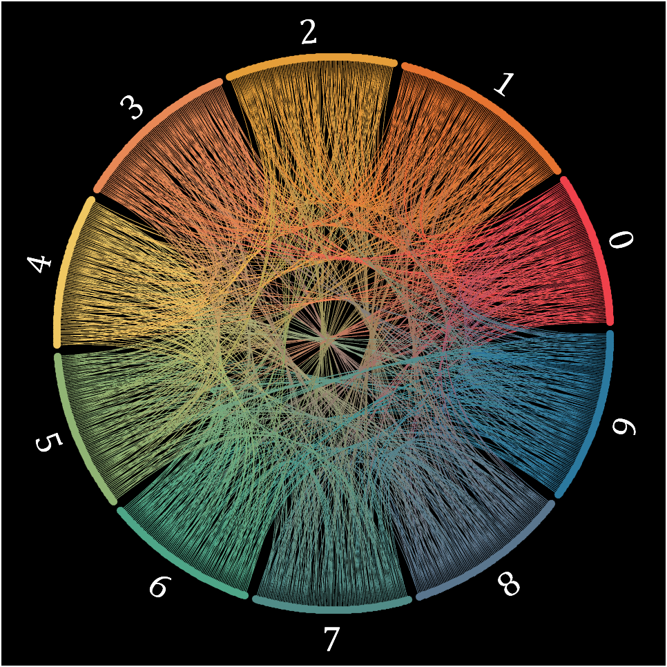
Class=getPi(1001)+1;
Data=diag(ones(1,1000),-1);
className={'0','1','2','3','4','5','6','7','8','9'};
colorOrder=[239,65,75;230,115,48;229,158,57;232,136,85;239,199,97;
144,180,116;78,166,136;81,140,136;90,118,142;43,121,159]./255;
CC=circosChart(Data,Class,'ClassName',className,'ColorOrder',colorOrder);
CC=CC.draw();
ax=gca;
ax.Color=[0,0,0];
CC.setClassLabel('Color',[1,1,1],'FontSize',25,'FontName','Cambria')
CC.setLine('LineWidth',.7)
YOU CAN GET ALL CODE HERE:
Given a vector v whose order we would like to randomly permute, many would perform the permutation by explicitly querying the length/size of v, e.g.,
I=randperm(numel(v));
v=v(I);
However, one can instead do as follows, avoiding the size query.
v=v(randperm(end))
Analogous things can be done with matrices, e.g.,
A=A(randperm(end), randperm(end));
code is here
You can also see the animated version of the competition here
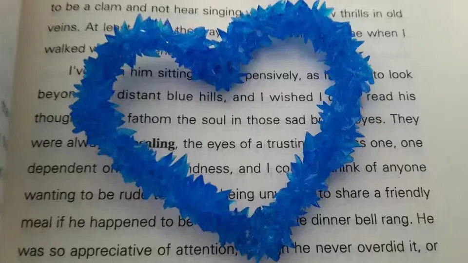
The creativity comes from the copper sulfate crystal heart made in junior high school. Copper sulfate is a triclinic crystal, and the same structure was not used here for convenience in drawing.
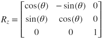
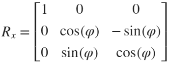
Part 1. Coordinate transformation
To draw a crystal heart, one must first be able to draw crystal clusters. To draw a crystal cluster, one must first be able to draw a crystal. To draw a crystal, we need this kind of structure:
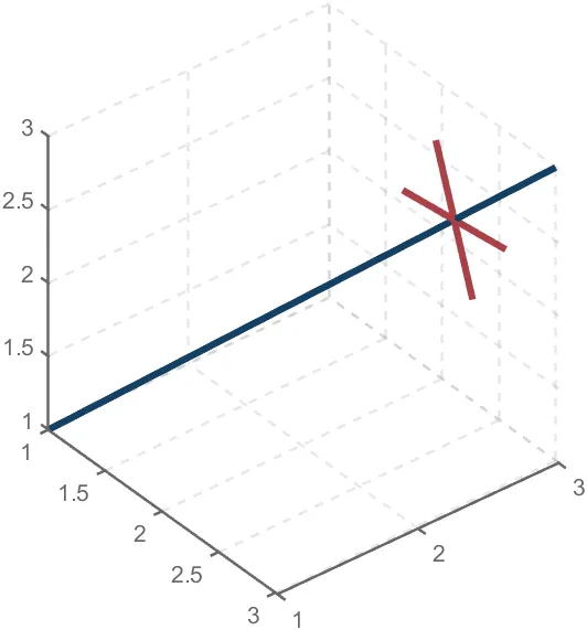
We first need a point with a certain distance from the straight line and a perpendicular point of cutPnt, which is very easy to find, for example, cutPnt=[x0, y0, z0]; The direction of the central axis is V=[x1, y1, z1]; If the distance to the straight line is L, the following points clearly meet the conditions:
v2=[z1,z1,-x1-y1];
v2=v2./norm(v2).*L;
pnt=cutPnt+v2;
But finding only one point is not enough. We need to find four points, and each point is obtained by rotating the previous point around a straight line by  degrees. Therefore, we need to obtain our point rotation transformation matrix around a straight line
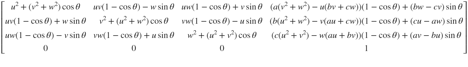
quite complex,right?
rotateMat=[u^2+(v^2+w^2)*cos(theta) , u*v*(1-cos(theta))-w*sin(theta), u*w*(1-cos(theta))+v*sin(theta), (a*(v^2+w^2)-u*(b*v+c*w))*(1-cos(theta))+(b*w-c*v)*sin(theta);
u*v*(1-cos(theta))+w*sin(theta), v^2+(u^2+w^2)*cos(theta) , v*w*(1-cos(theta))-u*sin(theta), (b*(u^2+w^2)-v*(a*u+c*w))*(1-cos(theta))+(c*u-a*w)*sin(theta);
u*w*(1-cos(theta))-v*sin(theta), v*w*(1-cos(theta))+u*sin(theta), w^2+(u^2+v^2)*cos(theta) , (c*(u^2+v^2)-w*(a*u+b*v))*(1-cos(theta))+(a*v-b*u)*sin(theta);
0 , 0 , 0 , 1];
Where [u, v, w] is the directional unit vector, and [a, b, c] is the initial coordinate of the axis:
Part 2. Crystal Cluster Drawing
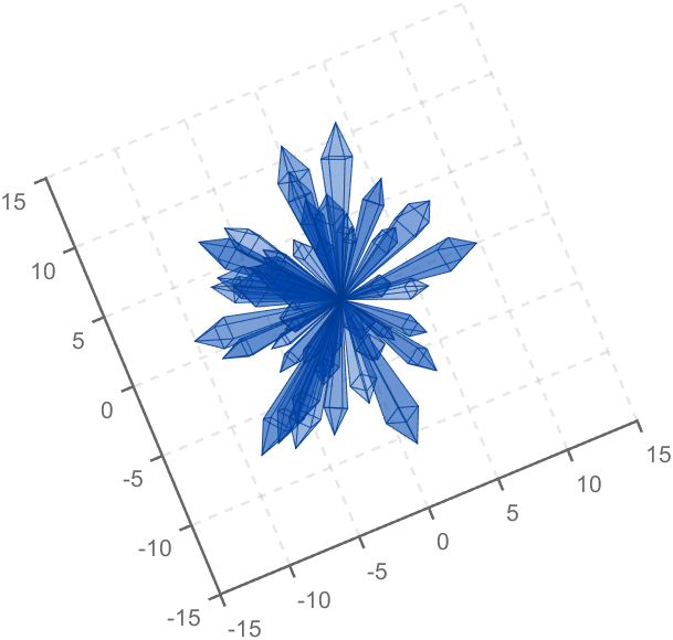
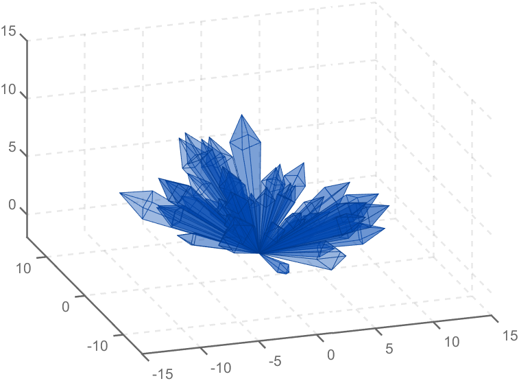
function crystall
hold on
for i=1:50
len=rand(1)*8+5;
tempV=rand(1,3)-0.5;
tempV(3)=abs(tempV(3));
tempV=tempV./norm(tempV).*len;
tempEpnt=tempV;
drawCrystal([0 0 0],tempEpnt,pi/6,0.8,0.1,rand(1).*0.2+0.2)
disp(i)
end
ax=gca;
ax.XLim=[-15,15];
ax.YLim=[-15,15];
ax.ZLim=[-2,15];
grid on
ax.GridLineStyle='--';
ax.LineWidth=1.2;
ax.XColor=[1,1,1].*0.4;
ax.YColor=[1,1,1].*0.4;
ax.ZColor=[1,1,1].*0.4;
ax.DataAspectRatio=[1,1,1];
ax.DataAspectRatioMode='manual';
ax.CameraPosition=[-67.6287 -204.5276 82.7879];
function drawCrystal(Spnt,Epnt,theta,cl,w,alpha)
%plot3([Spnt(1),Epnt(1)],[Spnt(2),Epnt(2)],[Spnt(3),Epnt(3)])
mainV=Epnt-Spnt;
cutPnt=cl.*(mainV)+Spnt;
cutV=[mainV(3),mainV(3),-mainV(1)-mainV(2)];
cutV=cutV./norm(cutV).*w.*norm(mainV);
cornerPnt=cutPnt+cutV;
cornerPnt=rotateAxis(Spnt,Epnt,cornerPnt,theta);
cornerPntSet(1,:)=cornerPnt';
for ii=1:3
cornerPnt=rotateAxis(Spnt,Epnt,cornerPnt,pi/2);
cornerPntSet(ii+1,:)=cornerPnt';
end
F = [1,3,4;1,4,5;1,5,6;1,6,3;...
2,3,4;2,4,5;2,5,6;2,6,3];
V = [Spnt;Epnt;cornerPntSet];
patch('Faces',F,'Vertices',V,'FaceColor',[0 71 177]./255,...
'FaceAlpha',alpha,'EdgeColor',[0 71 177]./255.*0.8,...
'EdgeAlpha',0.6,'LineWidth',0.5,'EdgeLighting',...
'gouraud','SpecularStrength',0.3)
end
function newPnt=rotateAxis(Spnt,Epnt,cornerPnt,theta)
V=Epnt-Spnt;V=V./norm(V);
u=V(1);v=V(2);w=V(3);
a=Spnt(1);b=Spnt(2);c=Spnt(3);
cornerPnt=[cornerPnt(:);1];
rotateMat=[u^2+(v^2+w^2)*cos(theta) , u*v*(1-cos(theta))-w*sin(theta), u*w*(1-cos(theta))+v*sin(theta), (a*(v^2+w^2)-u*(b*v+c*w))*(1-cos(theta))+(b*w-c*v)*sin(theta);
u*v*(1-cos(theta))+w*sin(theta), v^2+(u^2+w^2)*cos(theta) , v*w*(1-cos(theta))-u*sin(theta), (b*(u^2+w^2)-v*(a*u+c*w))*(1-cos(theta))+(c*u-a*w)*sin(theta);
u*w*(1-cos(theta))-v*sin(theta), v*w*(1-cos(theta))+u*sin(theta), w^2+(u^2+v^2)*cos(theta) , (c*(u^2+v^2)-w*(a*u+b*v))*(1-cos(theta))+(a*v-b*u)*sin(theta);
0 , 0 , 0 , 1];
newPnt=rotateMat*cornerPnt;
newPnt(4)=[];
end
end
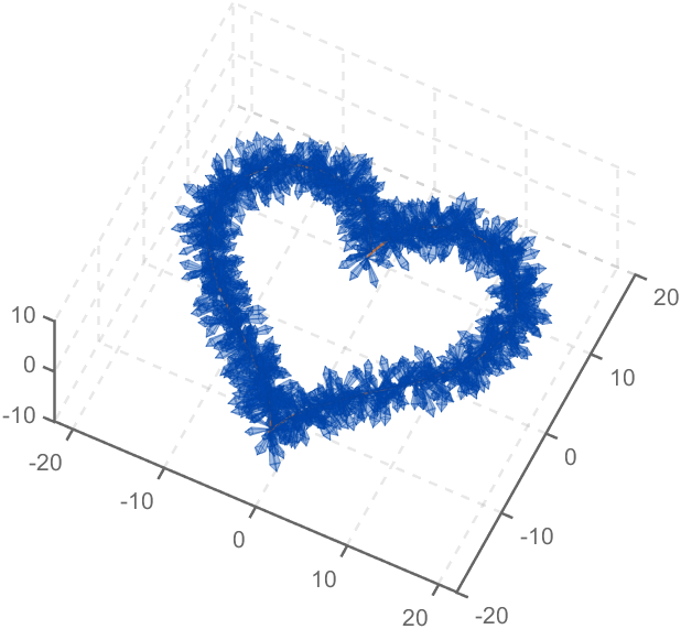
Part 3. Drawing of Crystal Heart
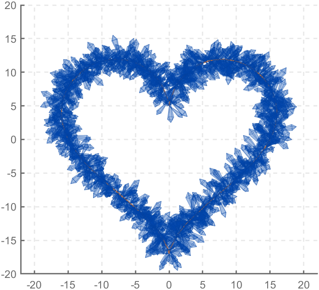
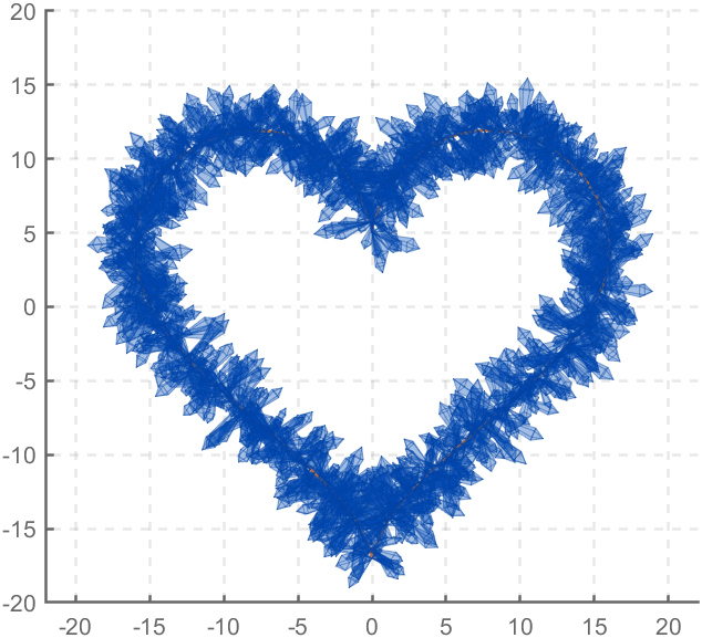
function crystalHeart
clc;clear;close all
hold on
% drawCrystal([1,1,1],[3,3,3],pi/6,0.8,0.14)
sep=pi/8;
t=[0:0.2:sep,sep:0.02:pi-sep,pi-sep:0.2:pi+sep,pi+sep:0.02:2*pi-sep,2*pi-sep:0.2:2*pi];
x=16*sin(t).^3;
y=13*cos(t)-5*cos(2*t)-2*cos(3*t)-cos(4*t);
z=zeros(size(t));
plot3(x,y,z,'Color',[186,110,64]./255,'LineWidth',1)
for i=1:length(t)
for j=1:6
len=rand(1)*2.5+1.5;
tempV=rand(1,3)-0.5;
tempV=tempV./norm(tempV).*len;
tempSpnt=[x(i),y(i),z(i)];
tempEpnt=tempV+tempSpnt;
drawCrystal(tempSpnt,tempEpnt,pi/6,0.8,0.14)
disp([i,j])
end
end
ax=gca;
ax.XLim=[-22,22];
ax.YLim=[-20,20];
ax.ZLim=[-10,10];
grid on
ax.GridLineStyle='--';
ax.LineWidth=1.2;
ax.XColor=[1,1,1].*0.4;
ax.YColor=[1,1,1].*0.4;
ax.ZColor=[1,1,1].*0.4;
ax.DataAspectRatio=[1,1,1];
ax.DataAspectRatioMode='manual';
function drawCrystal(Spnt,Epnt,theta,cl,w)
%plot3([Spnt(1),Epnt(1)],[Spnt(2),Epnt(2)],[Spnt(3),Epnt(3)])
mainV=Epnt-Spnt;
cutPnt=cl.*(mainV)+Spnt;
cutV=[mainV(3),mainV(3),-mainV(1)-mainV(2)];
cutV=cutV./norm(cutV).*w.*norm(mainV);
cornerPnt=cutPnt+cutV;
cornerPnt=rotateAxis(Spnt,Epnt,cornerPnt,theta);
cornerPntSet(1,:)=cornerPnt';
for ii=1:3
cornerPnt=rotateAxis(Spnt,Epnt,cornerPnt,pi/2);
cornerPntSet(ii+1,:)=cornerPnt';
end
F = [1,3,4;1,4,5;1,5,6;1,6,3;...
2,3,4;2,4,5;2,5,6;2,6,3];
V = [Spnt;Epnt;cornerPntSet];
patch('Faces',F,'Vertices',V,'FaceColor',[0 71 177]./255,...
'FaceAlpha',0.2,'EdgeColor',[0 71 177]./255.*0.9,...
'EdgeAlpha',0.25,'LineWidth',0.01,'EdgeLighting',...
'gouraud','SpecularStrength',0.3)
end
function newPnt=rotateAxis(Spnt,Epnt,cornerPnt,theta)
V=Epnt-Spnt;V=V./norm(V);
u=V(1);v=V(2);w=V(3);
a=Spnt(1);b=Spnt(2);c=Spnt(3);
cornerPnt=[cornerPnt(:);1];
rotateMat=[u^2+(v^2+w^2)*cos(theta) , u*v*(1-cos(theta))-w*sin(theta), u*w*(1-cos(theta))+v*sin(theta), (a*(v^2+w^2)-u*(b*v+c*w))*(1-cos(theta))+(b*w-c*v)*sin(theta);
u*v*(1-cos(theta))+w*sin(theta), v^2+(u^2+w^2)*cos(theta) , v*w*(1-cos(theta))-u*sin(theta), (b*(u^2+w^2)-v*(a*u+c*w))*(1-cos(theta))+(c*u-a*w)*sin(theta);
u*w*(1-cos(theta))-v*sin(theta), v*w*(1-cos(theta))+u*sin(theta), w^2+(u^2+v^2)*cos(theta) , (c*(u^2+v^2)-w*(a*u+b*v))*(1-cos(theta))+(a*v-b*u)*sin(theta);
0 , 0 , 0 , 1];
newPnt=rotateMat*cornerPnt;
newPnt(4)=[];
end
end
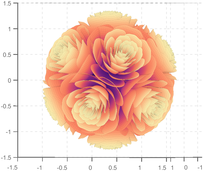
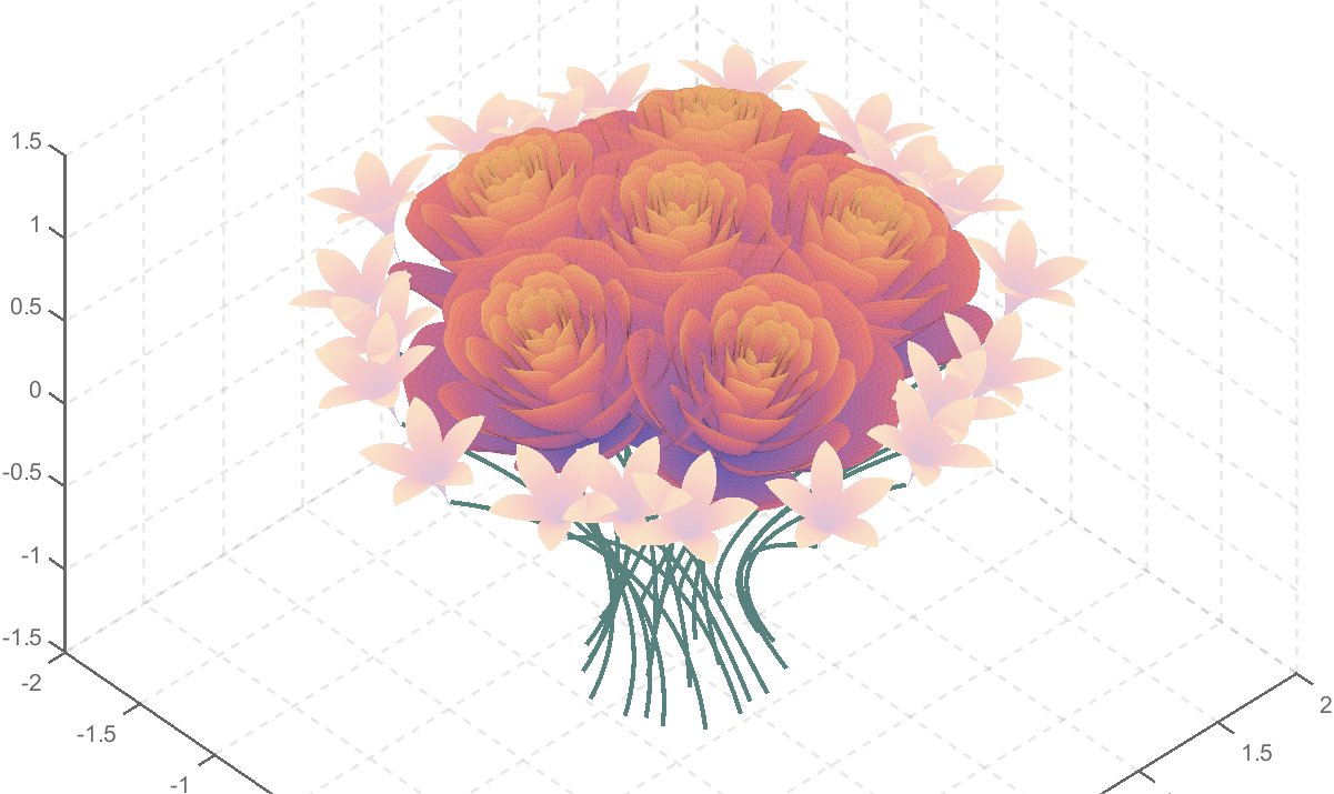
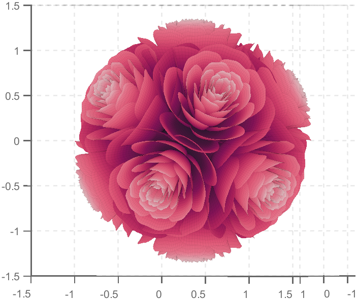
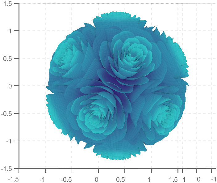
So, how to draw a roseball just like this ?
To begin with, we need to know how to draw a single rose in MATLAB:
function drawrose
set(gca,'CameraPosition',[2 2 2])
hold on
grid on
[x,t]=meshgrid((0:24)./24,(0:0.5:575)./575.*20.*pi+4*pi);
p=(pi/2)*exp(-t./(8*pi));
change=sin(15*t)/150;
u=1-(1-mod(3.6*t,2*pi)./pi).^4./2+change;
y=2*(x.^2-x).^2.*sin(p);
r=u.*(x.*sin(p)+y.*cos(p));
h=u.*(x.*cos(p)-y.*sin(p));
surface(r.*cos(t),r.*sin(t),h,'EdgeAlpha',0.1,...
'EdgeColor',[0 0 0],'FaceColor','interp')
end
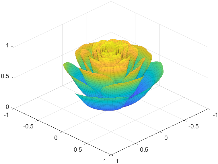
Tts pretty easy, Now we are trying to dye it the desired color:
function drawrose
set(gca,'CameraPosition',[2 2 2])
hold on
grid on
[x,t]=meshgrid((0:24)./24,(0:0.5:575)./575.*20.*pi+4*pi);
p=(pi/2)*exp(-t./(8*pi));
change=sin(15*t)/150;
u=1-(1-mod(3.6*t,2*pi)./pi).^4./2+change;
y=2*(x.^2-x).^2.*sin(p);
r=u.*(x.*sin(p)+y.*cos(p));
h=u.*(x.*cos(p)-y.*sin(p));
map=[0.9176 0.9412 1.0000
0.8353 0.8706 0.9922
0.8196 0.8627 0.9804
0.7020 0.7569 0.9412
0.5176 0.5882 0.9255
0.3686 0.4824 0.9412
0.3059 0.4000 0.9333
0.2275 0.3176 0.8353
0.1216 0.2275 0.6471];
Xi=1:size(map,1);Xq=linspace(1,size(map,1),100);
map=[interp1(Xi,map(:,1),Xq,'linear')',...
interp1(Xi,map(:,2),Xq,'linear')',...
interp1(Xi,map(:,3),Xq,'linear')'];
surface(r.*cos(t),r.*sin(t),h,'EdgeAlpha',0.1,...
'EdgeColor',[0 0 0],'FaceColor','interp')
colormap(map)
end
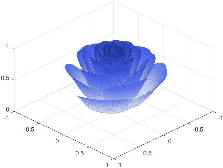
I try to take colors from real roses and interpolate them to make them more realistic
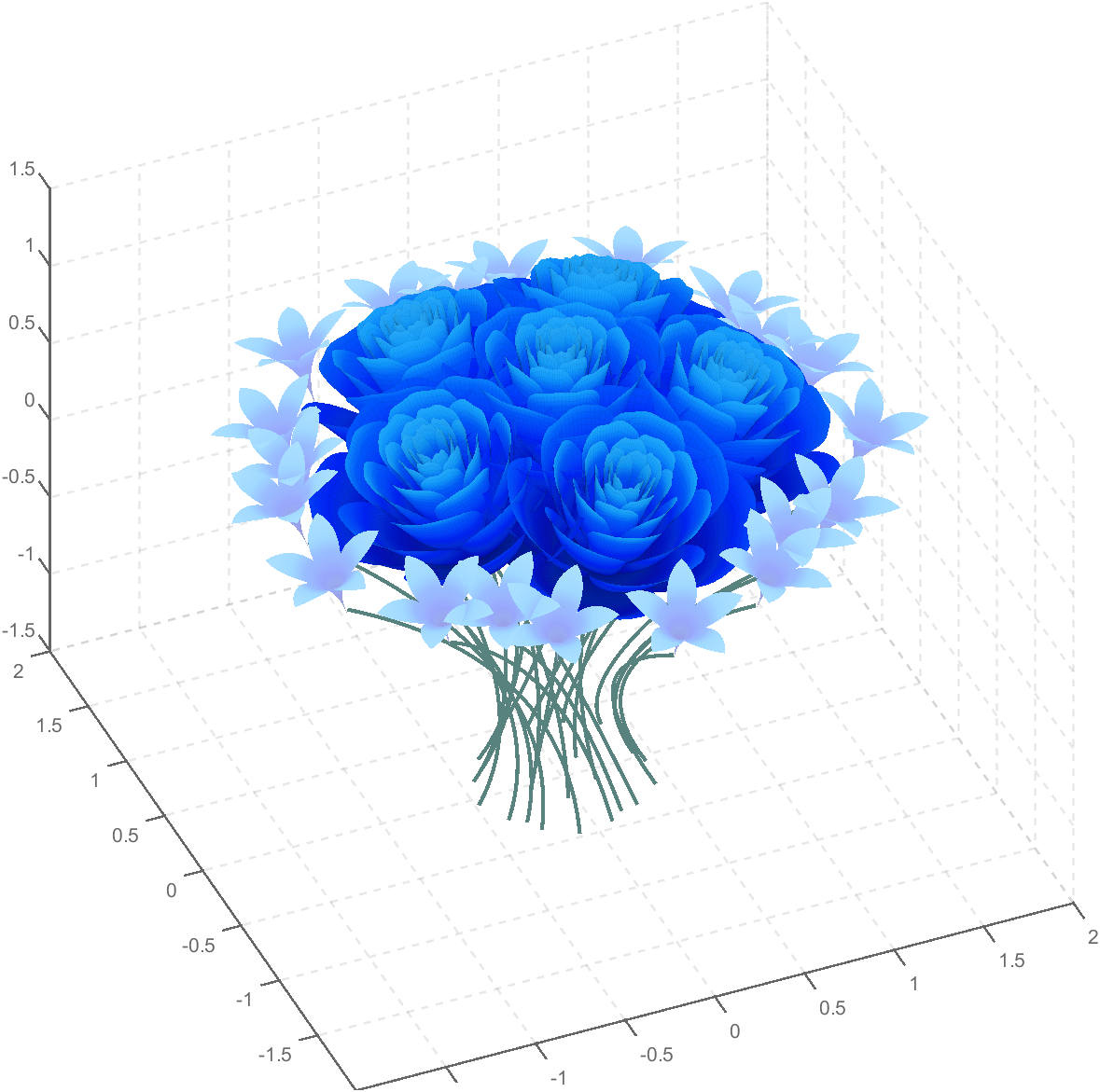
Then, how can I put these colorful flowers on to a ball ?
We need to place the drawn flowers on each face of the polyhedron sphere through coordinate transformation. Here, we use a regular dodecahedron:
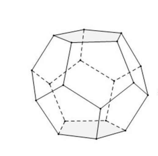
Move the flower using the following rotation formula:
We place a flower on each plane, which means that the angle between every two flowers is  degrees. We can place each flower at the appropriate angle through multiple x-axis rotations and multiple z-axis rotations. The code is as follows:
function roseBall(colorList)
%曲面数据计算
%==========================================================================
[x,t]=meshgrid((0:24)./24,(0:0.5:575)./575.*20.*pi+4*pi);
p=(pi/2)*exp(-t./(8*pi));
change=sin(15*t)/150;
u=1-(1-mod(3.6*t,2*pi)./pi).^4./2+change;
y=2*(x.^2-x).^2.*sin(p);
r=u.*(x.*sin(p)+y.*cos(p));
h=u.*(x.*cos(p)-y.*sin(p));
%颜色映射表
%==========================================================================
hMap=(h-min(min(h)))./(max(max(h))-min(min(h)));
col=size(hMap,2);
if nargin<1
colorList=[0.0200 0.0400 0.3900
0 0.0900 0.5800
0 0.1300 0.6400
0.0200 0.0600 0.6900
0 0.0800 0.7900
0.0100 0.1800 0.8500
0 0.1300 0.9600
0.0100 0.2600 0.9900
0 0.3500 0.9900
0.0700 0.6200 1.0000
0.1700 0.6900 1.0000];
end
colorFunc=colorFuncFactory(colorList);
dataMap=colorFunc(hMap');
colorMap(:,:,1)=dataMap(:,1:col);
colorMap(:,:,2)=dataMap(:,col+1:2*col);
colorMap(:,:,3)=dataMap(:,2*col+1:3*col);
function colorFunc=colorFuncFactory(colorList)
xx=(0:size(colorList,1)-1)./(size(colorList,1)-1);
y1=colorList(:,1);y2=colorList(:,2);y3=colorList(:,3);
colorFunc=@(X)[interp1(xx,y1,X,'linear')',interp1(xx,y2,X,'linear')',interp1(xx,y3,X,'linear')'];
end
%曲面旋转及绘制
%==========================================================================
surface(r.*cos(t),r.*sin(t),h+0.35,'EdgeAlpha',0.05,...
'EdgeColor',[0 0 0],'FaceColor','interp','CData',colorMap)
hold on
surface(r.*cos(t),r.*sin(t),-h-0.35,'EdgeAlpha',0.05,...
'EdgeColor',[0 0 0],'FaceColor','interp','CData',colorMap)
Xset=r.*cos(t);
Yset=r.*sin(t);
Zset=h+0.35;
yaw_z=72*pi/180;
roll_x=pi-acos(-1/sqrt(5));
R_z_2=[cos(yaw_z),-sin(yaw_z),0;
sin(yaw_z),cos(yaw_z),0;
0,0,1];
R_z_1=[cos(yaw_z/2),-sin(yaw_z/2),0;
sin(yaw_z/2),cos(yaw_z/2),0;
0,0,1];
R_x_2=[1,0,0;
0,cos(roll_x),-sin(roll_x);
0,sin(roll_x),cos(roll_x)];
[nX,nY,nZ]=rotateXYZ(Xset,Yset,Zset,R_x_2);
surface(nX,nY,nZ,'EdgeAlpha',0.05,...
'EdgeColor',[0 0 0],'FaceColor','interp','CData',colorMap)
for k=1:4
[nX,nY,nZ]=rotateXYZ(nX,nY,nZ,R_z_2);
surface(nX,nY,nZ,'EdgeAlpha',0.05,...
'EdgeColor',[0 0 0],'FaceColor','interp','CData',colorMap)
end
[nX,nY,nZ]=rotateXYZ(nX,nY,nZ,R_z_1);
for k=1:5
[nX,nY,nZ]=rotateXYZ(nX,nY,nZ,R_z_2);
surface(nX,nY,-nZ,'EdgeAlpha',0.05,...
'EdgeColor',[0 0 0],'FaceColor','interp','CData',colorMap)
end
%--------------------------------------------------------------------------
function [nX,nY,nZ]=rotateXYZ(X,Y,Z,R)
nX=zeros(size(X));
nY=zeros(size(Y));
nZ=zeros(size(Z));
for i=1:size(X,1)
for j=1:size(X,2)
v=[X(i,j);Y(i,j);Z(i,j)];
nv=R*v;
nX(i,j)=nv(1);
nY(i,j)=nv(2);
nZ(i,j)=nv(3);
end
end
end
%axes属性调整
%==========================================================================
ax=gca;
grid on
ax.GridLineStyle='--';
ax.LineWidth=1.2;
ax.XColor=[1,1,1].*0.4;
ax.YColor=[1,1,1].*0.4;
ax.ZColor=[1,1,1].*0.4;
ax.DataAspectRatio=[1,1,1];
ax.DataAspectRatioMode='manual';
ax.CameraPosition=[-6.5914 -24.1625 -0.0384];
end

TRY DIFFERENT COLORS !!
colorList1=[0.2000 0.0800 0.4300
0.2000 0.1300 0.4600
0.2000 0.2100 0.5000
0.2000 0.2800 0.5300
0.2000 0.3700 0.5800
0.1900 0.4500 0.6200
0.2000 0.4800 0.6400
0.1900 0.5400 0.6700
0.1900 0.5700 0.6900
0.1900 0.7500 0.7800
0.1900 0.8000 0.8100
];
colorList2=[0.1300 0.1000 0.1600
0.2000 0.0900 0.2000
0.2800 0.0800 0.2300
0.4200 0.0800 0.3000
0.5100 0.0700 0.3400
0.6600 0.1200 0.3500
0.7900 0.2200 0.4000
0.8800 0.3500 0.4700
0.9000 0.4500 0.5400
0.8900 0.7800 0.7900
];
colorList3=[0.3200 0.3100 0.7600
0.3800 0.3400 0.7600
0.5300 0.4200 0.7500
0.6400 0.4900 0.7300
0.7200 0.5500 0.7200
0.7900 0.6100 0.7100
0.9100 0.7100 0.6800
0.9800 0.7600 0.6700
];
colorList4=[0.2100 0.0900 0.3800
0.2900 0.0700 0.4700
0.4000 0.1100 0.4900
0.5500 0.1600 0.5100
0.7500 0.2400 0.4700
0.8900 0.3200 0.4100
0.9700 0.4900 0.3700
1.0000 0.5600 0.4100
1.0000 0.6900 0.4900
1.0000 0.8200 0.5900
0.9900 0.9200 0.6700
0.9800 0.9500 0.7100];
Let us consider how to draw a Happy Sheep. A Happy Sheep was introduced in the MATLAB Mini Hack contest: Happy Sheep!
In this contest there was the strict limitation on the code length. So the code of the Happy Sheep is very compact and is only 280 characters long. We will analyze the process of drawing the Happy Sheep in MATLAB step by step. The explanations of the even more compact version of the code of the same sheep are given below.
So, how to draw a sheep? It is very easy. We could notice that usually a sheep is covered by crimped wool. Therefore, a sheep could be painted using several geometrical curves of similar types. Of course, then it will be an abstract model of the real sheep. Let us select two mathematical curves, which are the most appropriate for our goal. They are an ellipse for smooth parts of the sheep and an ellipse combined with a rose for woolen parts of the sheep.
Let us recall the mathematical formulas of these curves. A parametric representation of the standard ellipse is the following:
Also we will use the following parametric representation of the rose (rhodonea) curve:
This curve was named by the mathematician Guido Grandi.
Let us combine them in one curve and add possible shifts:
Now if we would like to create an ellipse, we will set  and
and  . If we would like to create a rose, we will set
  and
and  . If we would like to shift our curve, we will set
  and
and  to the required values. Of course, we could set all non-zero parameters to combine both chosen curves and use the shifts.
Let us describe how to create these curves using the MATLAB code. To make the code more compact, it is possible to program both formulas for the combined curve in one line using the anonymous function. We could make the code more compact using the function handles for sine and cosine functions. Then the MATLAB code for an example of the ellipse curve will be the following.
% Handles
s=@sin;
c=@cos;
% Ellipse + Polar Rose
F=@(t,a,f) a(1)*f(t)+s(a(2)*t).*f(t)+a(3);
% Angles
t=0:.1:7;
% Parameters
E = [5 7;0 0;0 0];
% Painting
figure;
plot(F(t,E(:,1),c),F(t,E(:,2),s),'LineWidth',10);
axis equal
The parameter t varies from 0 to 7, which is the nearest integer greater than  , with the step 0.1. The result of this code is the following ellipse curve with
  and
and  .
.
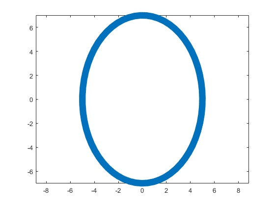
This ellipse is described by the following parametric equations:
The MATLAB code for an example of the rose curve will be the following.
% Handles
s=@sin;
c=@cos;
% Ellipse + Polar Rose
F=@(t,a,f) a(1)*f(t)+s(a(2)*t).*f(t)+a(3);
% Angles
t=0:.1:7;
% Parameters
R = [0 0;4 4;0 0];
% Painting
figure;
plot(F(t,R(:,1),c),F(t,R(:,2),s),'LineWidth',10);
axis equal
The result of this code is the following rose curve with  and
and  .
.
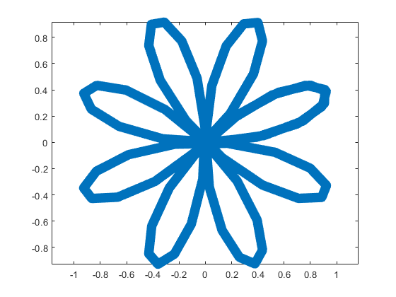
This rose is described by the following parametric equations:
Obviously, now we are ready to draw main parts of our sheep! As we reproduce an abstract model of the sheep, let us select the following main parts for the representation: head, eyes, hoofs, body, crown, and tail. We will use ellipses for the first three parts in this list and ellipses combined with roses for the last three ones.
First let us describe drawing of each part independently.
The following MATLAB code will be used to do this.
% Handles
s=@sin;
c=@cos;
% Ellipse + Polar Rose
F=@(t,a,f) a(1)*f(t)+s(a(2)*t).*f(t)+a(3);
% Angles
t=0:.1:7;
% Parameters
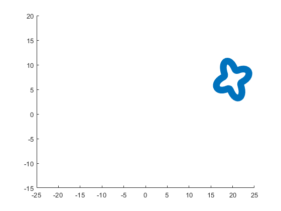
Head = 1;
Eyes = 2:3;
Hoofs = 4:7;
Body = 8;
Crown = 9;
Tail = 10;
G=-13;
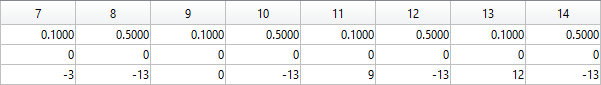
P=[5 7 repmat([.1 .5],1,6) 6 4 14 9 3 3;zeros(1,14) 8 8 12 12 4 4;...
-15 2 G 3 -17 3 -3 G 0 G 9 G 12 G -15 12 4 3 20 7];
% Painting
figure;
hold;
for i=Head
plot(F(t,P(:,2*i-1),c),F(t,P(:,2*i),s),'LineWidth',10);
end
axis([-25 25 -15 20]);
figure;
hold;
for i=Eyes
plot(F(t,P(:,2*i-1),c),F(t,P(:,2*i),s),'LineWidth',10);
end
axis([-25 25 -15 20]);
figure;
hold;
for i=Hoofs
plot(F(t,P(:,2*i-1),c),F(t,P(:,2*i),s),'LineWidth',10);
end
axis([-25 25 -15 20]);
figure;
hold;
for i=Body
plot(F(t,P(:,2*i-1),c),F(t,P(:,2*i),s),'LineWidth',10);
end
axis([-25 25 -15 20]);
figure;
hold;
for i=Crown
plot(F(t,P(:,2*i-1),c),F(t,P(:,2*i),s),'LineWidth',10);
end
axis([-25 25 -15 20]);
figure;
hold;
for i=Tail
plot(F(t,P(:,2*i-1),c),F(t,P(:,2*i),s),'LineWidth',10);
end
axis([-25 25 -15 20]);
The parameters  ,
,  ,
,  ,
,  ,
,  , and
, and  are written in the different submatrices of the matrix P. The code generates the following curves to illustrate the different parts of our sheep.
The following ellipse describes the head of the sheep.
The following submatrix of the matrix P represents its parameters.
The parametric equations of the head are the following:
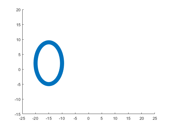
The following ellipses describe the eyes of the sheep.
The following submatrices of the matrix P represent their parameters.
The parametric equations of the left and right eyes correspondingly are the following:
The following ellipses describe the hoofs of the sheep.
The following submatrices of the matrix P represent their parameters.
The parametric equations of the right front, left front, right hind, and left hind hoofs correspondingly are the following:
The following ellipse combined with the rose describes the crown of the sheep.
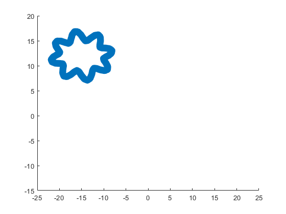
The following submatrix of the matrix P represents its parameters.
The parametric equations of the crown are the following:
The following ellipse combined with the rose describes the body of the sheep.
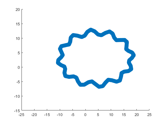
The following submatrix of the matrix P represents its parameters.
The parametric equations of the body are the following:
The following ellipse combined with the rose describes the tail of the sheep.
The following submatrix of the matrix P represents its parameters.
The parametric equations of the tail are the following:
Now all the parts of our sheep should be put together! It is very easy because all the parts are described by the same equations with different parameters.
The following code helps us to accomplish this goal and ultimately draw a Happy Sheep in MATLAB!
% Happy Sheep!
% By Victoria A. Sablina
% Handles
s=@sin;
c=@cos;
% Ellipse + Rose
F=@(t,a,f) a(1)*f(t)+s(a(2)*t).*f(t)+a(3);
% Angles
t=0:.1:7;
% Parameters
% Head (1:2)
% Eyes (3:6)
% Hoofs (7:14)
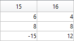
% Crown (15:16)
% Body (17:18)
% Tail (19:20)
G=-13;
P=[5 7 repmat([.1 .5],1,6) 6 4 14 9 3 3;zeros(1,14) 8 8 12 12 4 4;...
-15 2 G 3 -17 3 -3 G 0 G 9 G 12 G -15 12 4 3 20 7];
% Painting
hold;
for i=1:10
plot(F(t,P(:,2*i-1),c),F(t,P(:,2*i),s),'LineWidth',10);
end
This code is even more compact than the original code from the contest. It is only 253 instead of 280 characters long and generates the same Happy Sheep!
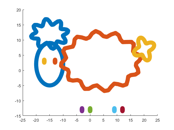
Our sheep is happy, because of becoming famous in the MATLAB community, a star!
Congratulations! Now you know how to draw a Happy Sheep in MATLAB!
Thank you for reading!
To enlarge an array with more rows and/or columns, you can set the lower right index to zero. This will pad the matrix with zeros.
m = rand(2, 3) % Initial matrix is 2 rows by 3 columns
mCopy = m;
% Now make it 2 rows by 5 columns
m(2, 5) = 0
m = mCopy; % Go back to original matrix.
% Now make it 3 rows by 3 columns
m(3, 3) = 0
m = mCopy; % Go back to original matrix.
% Now make it 3 rows by 7 columns
m(3, 7) = 0
MATLAB O/X Quiz
Answer BEFORE Googling!
- An infinite loop can be made using "for".
- "A == A" is always true.
- "round(2.5)" is 3.
- "round(-0.5)" is 0.
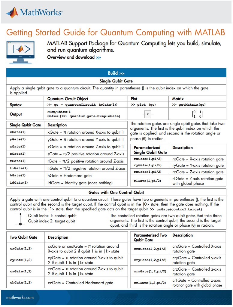
MATLAB Support Package for Quantum Computing lets you build, simulate, and run quantum algorithms.
Check out the Cheat Sheet here!
The MATLAB command window isn't just for commands and outputs—it can also host interactive hyperlinks. These can serve as powerful shortcuts, enhancing the feedback you provide during code execution. Here are some hyperlinks I frequently use in fprintf statements, warnings, or error messages.
1. Open a website.
msg = "Could not download data from website.";
url = "https://blogs.mathworks.com/graphics-and-apps/";
hypertext = "Go to website"
fprintf(1,'%s <a href="matlab: web(''%s'') ">%s</a>\n',msg,url,hypertext);
Could not download data from website. Go to website
2. Open a folder in file explorer (Windows)
msg = "File saved to current directory.";
directory = cd();
hypertext = "[Open directory]";
fprintf(1,'%s <a href="matlab: winopen(''%s'') ">%s</a>\n',msg,directory,hypertext)
File saved to current directory. [Open directory]
3. Open a document (Windows)
msg = "Created database.csv.";
filepath = fullfile(cd,'database.csv');
hypertext = "[Open file]";
fprintf(1,'%s <a href="matlab: winopen(''%s'') ">%s</a>\n',msg,filepath,hypertext)
Created database.csv. [Open file]
4. Open an m-file and go to a specific line
msg = 'Go to';
file = 'streamline.m';
line = 51;
fprintf(1,'%s <a href="matlab: matlab.desktop.editor.openAndGoToLine(which(''%s''), %d); ">%s line %d</a>', msg, file, line, file, line);
Go to streamline.m line 51
5. Display more text
msg = 'Incomplete data detected.';
extendedInfo = '\tFilename: m32c4r28\n\tDate: 12/20/2014\n\tElectrode: (3,7)\n\tDepth: ???\n';
hypertext = '[Click for more info]';
warning('%s <a href="matlab: fprintf(''%s'') ">%s</a>', msg,extendedInfo,hypertext);
<click>
- Filename: m32c4r28
- Date: 12/20/2014
- Electrode: (3,7)
- Depth: ???
6. Run a function
Similarly, you can also add hyperlinks in figures and apps
I would tell myself to understand vectorization. MATLAB is designed for operating on whole arrays and matrices at once. This is often more efficient than using loops.
and immeditaely everyone wanted the code! It turns out that this is the result of my remix of @Zhaoxu Liu / slandarer's entry on the MATLAB Flipbook Mini Hack.
I pointed people to the Flipbook entry but, of course, that just gave the code to render a single frame and people wanted the full code to render the animated gif. That way, they could make personalised versions
I just published a blog post that gives the code used by the team behind the Mini Hack to produce the animated .gifs https://blogs.mathworks.com/matlab/2024/02/16/producing-animated-gifs-from-matlab-flipbook-mini-hack-entries/
Thanks again to @Zhaoxu Liu / slandarer for a great entry that seems like it will live for a long time :)
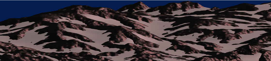
I think that MATLAB's Flipbook Mini Hack had quite some inspiring entries. My work largely deals with digital elevation models (DEMs). Hence I really liked the random renderings of landscapes, in particular this one written by Tim which inspired me to adopt the code and apply to the example data that comes with my software TopoToolbox. The results and code are shown here.
I found this list on Book Authority about the top MATLAB books: https://bookauthority.org/books/best-matlab-books
My favorite book is Accelerating MATLAB Performance - 1001 tips to speed up MATLAB programs. I always pick something up from the book that helps me out.
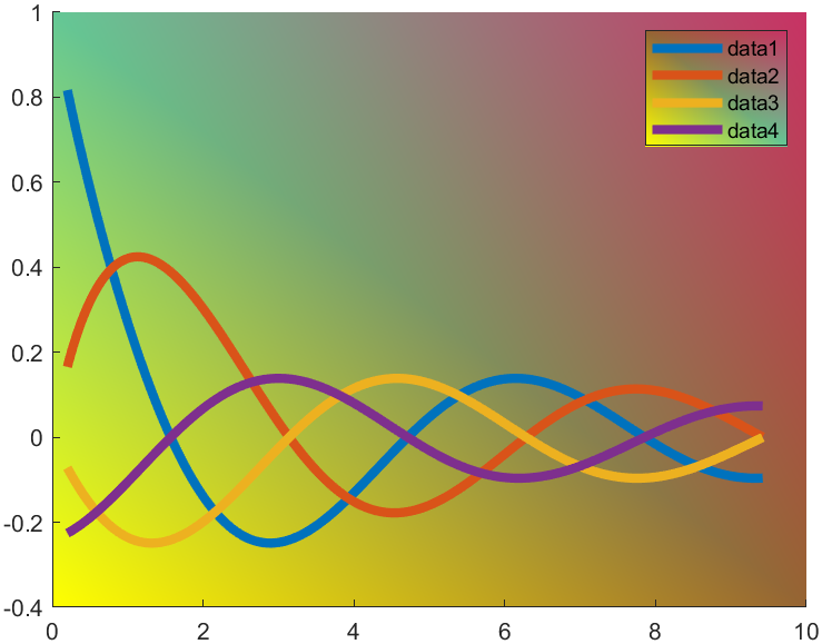
t=0.2:0.01:3*pi;
hold on
plot(t,cos(t)./(1+t),'LineWidth',4)
plot(t,sin(t)./(1+t),'LineWidth',4)
plot(t,cos(t+pi/2)./(1+t+pi/2),'LineWidth',4)
plot(t,cos(t+pi)./(1+t+pi),'LineWidth',4)
ax=gca;
hLegend=legend();
pause(1e-16)
colorData = uint8([255, 150, 200, 100; ...
255, 100, 50, 200; ...
0, 50, 100, 150; ...
102, 150, 200, 50]);
set(ax.Backdrop.Face, 'ColorBinding','interpolated','ColorData',colorData);
set(hLegend.BoxFace,'ColorBinding','interpolated','ColorData',colorData)
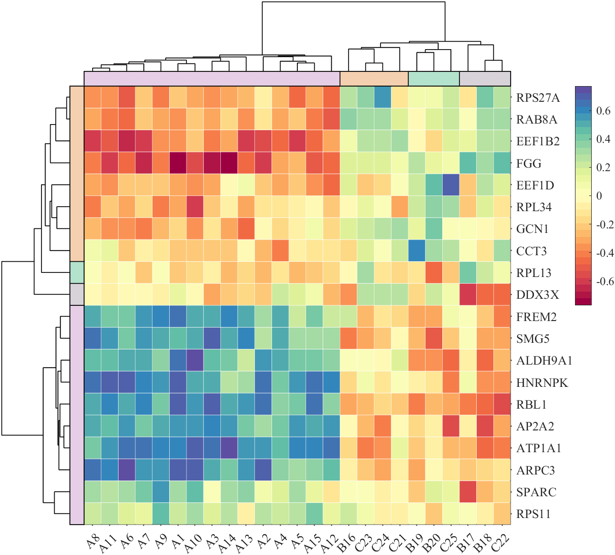
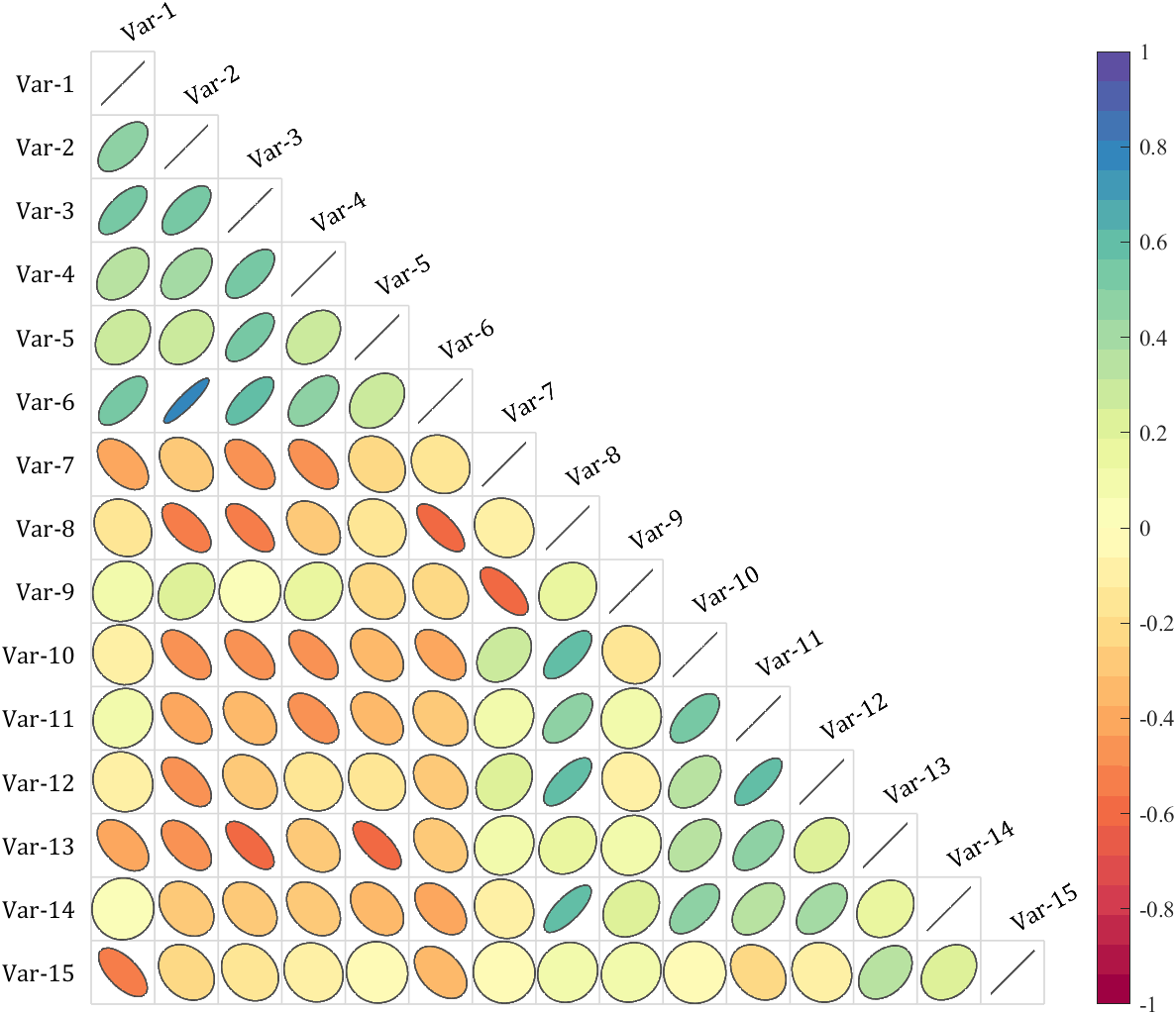
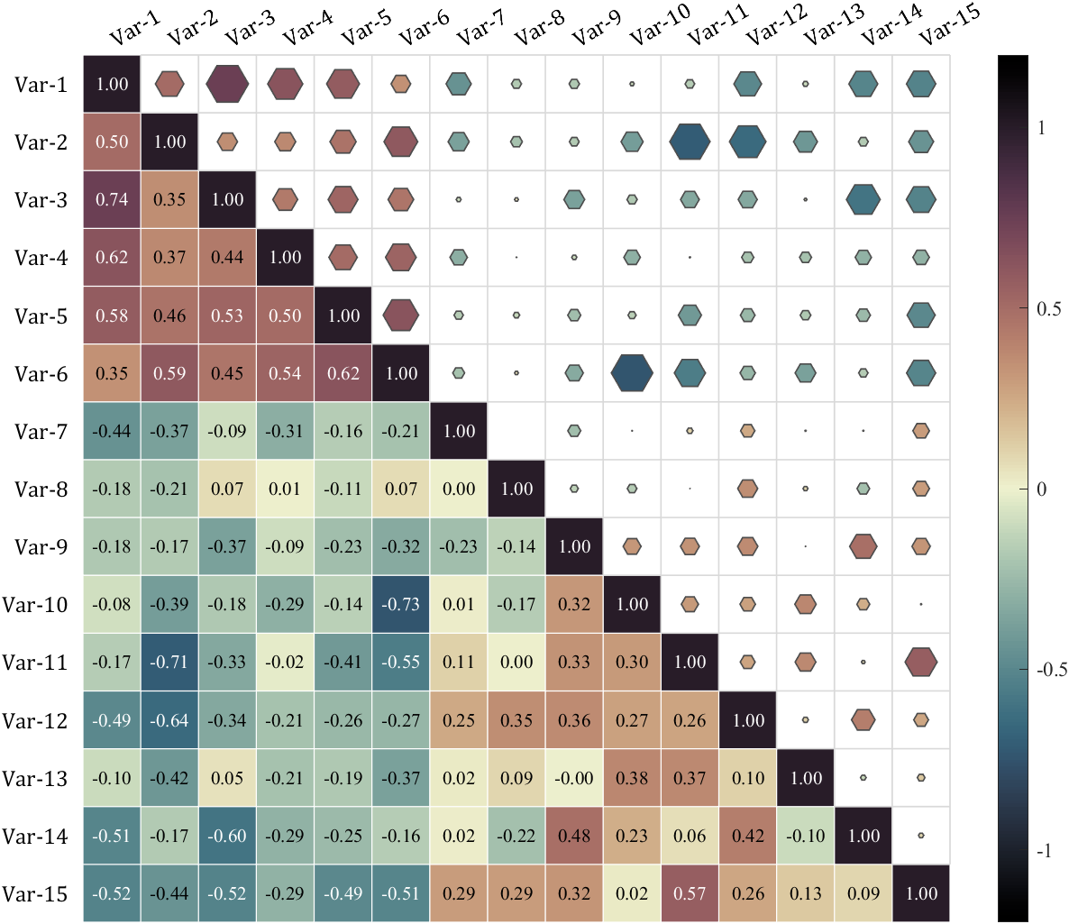
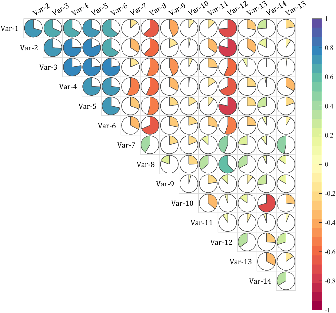
It is pretty easy to draw a cool heatmap for I have uploaded a tool to fileexchange:
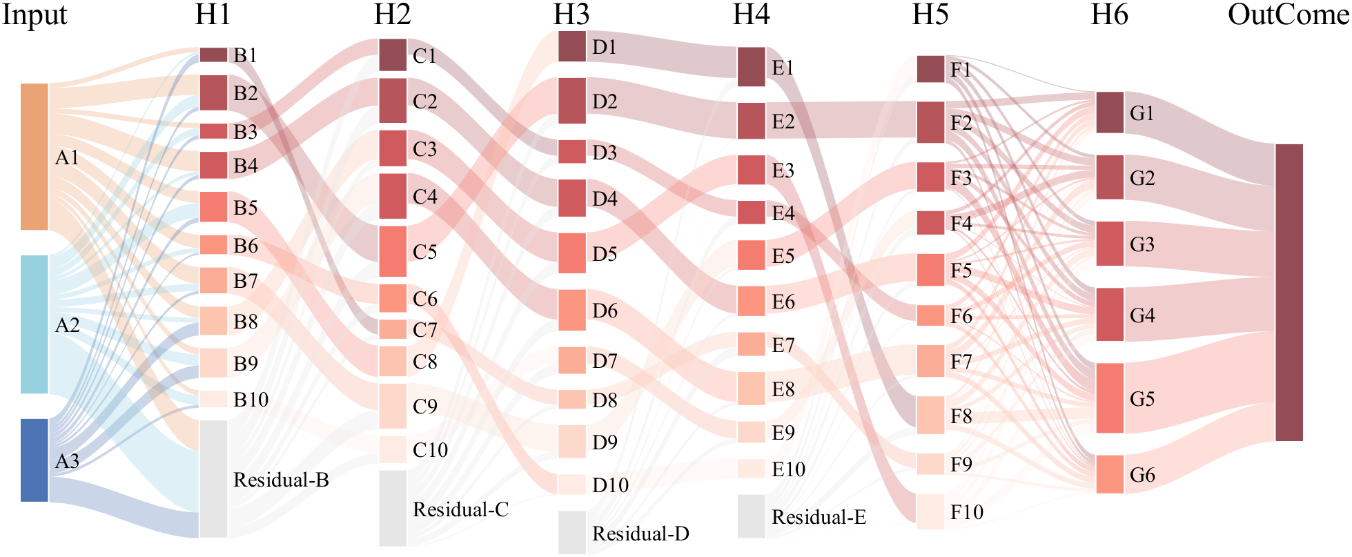
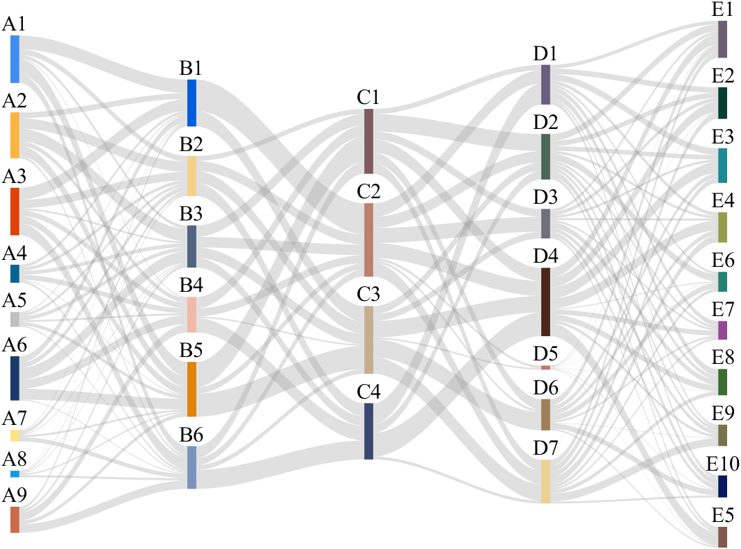
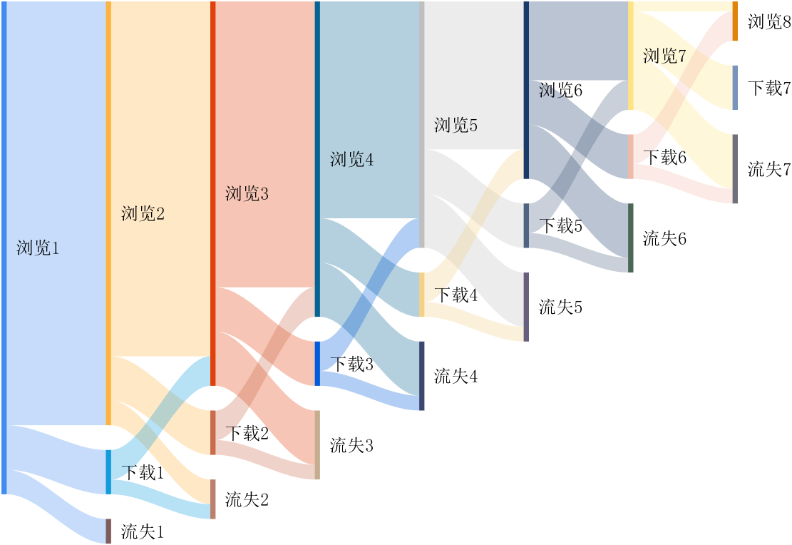
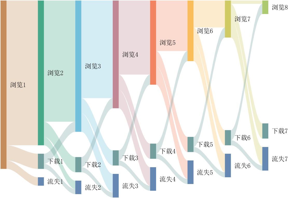
It is easy to obtain sankey plot like that using my tool:
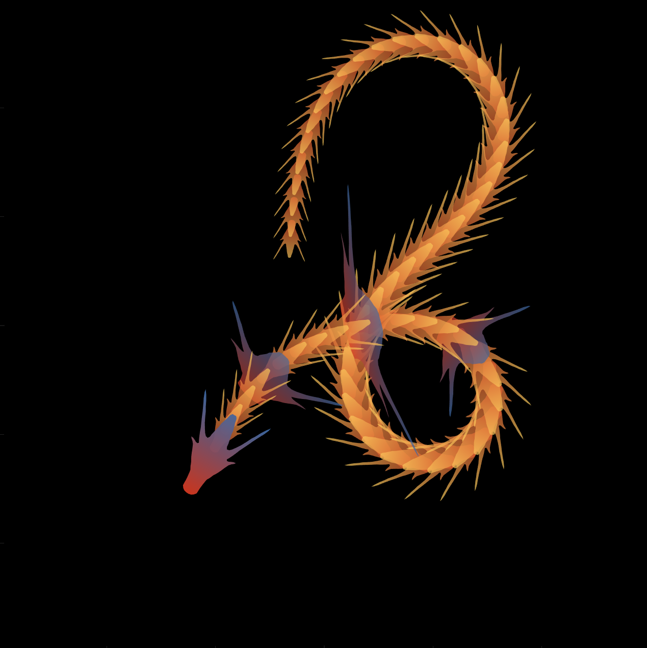
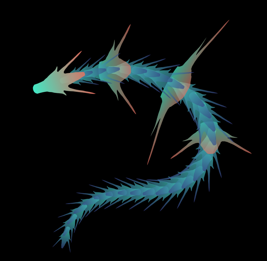
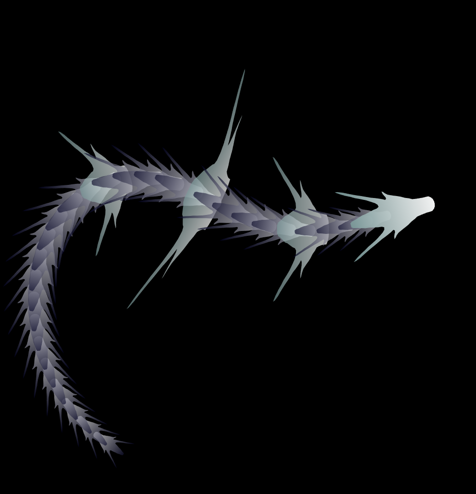
function dragon24
% Copyright (c) 2024, Zhaoxu Liu / slandarer
baseV=[ -.016,.822; -.074,.809; -.114,.781; -.147,.738; -.149,.687; -.150,.630;
-.157,.554; -.166,.482; -.176,.425; -.208,.368; -.237,.298; -.284,.216;
-.317,.143; -.338,.091; -.362,.037;-.382,-.006;-.420,-.051;-.460,-.084;
-.477,-.110;-.430,-.103;-.387,-.084;-.352,-.065;-.317,-.060;-.300,-.082;
-.331,-.139;-.359,-.201;-.385,-.262;-.415,-.342;-.451,-.418;-.494,-.510;
-.533,-.599;-.569,-.675;-.607,-.753;-.647,-.829;-.689,-.932;-.699,-.988;
-.639,-.905;-.581,-.809;-.534,-.717;-.489,-.642;-.442,-.543;-.393,-.447;
-.339,-.362;-.295,-.296;-.251,-.251;-.206,-.241;-.183,-.281;-.175,-.350;
-.156,-.434;-.136,-.521;-.128,-.594;-.103,-.677;-.083,-.739;-.067,-.813;-.039,-.852];
% 基础比例、上色方式数据
baseV=[0,.82;baseV;baseV(end:-1:1,:).*[-1,1];0,.82];
baseV=baseV-mean(baseV,1);
baseF=1:size(baseV,1);
baseY=baseV(:,2);
baseY=(baseY-min(baseY))./(max(baseY)-min(baseY));
N=30;
baseR=sin(linspace(pi/4,5*pi/6,N))./1.2;
baseR=[baseR',baseR'];baseR(1,:)=[1,1];
baseR(5,:)=[2,.6];
baseR(10,:)=[3.7,.4];
baseR(15,:)=[1.8,.6];
baseT=[zeros(N,1),ones(N,1)];
baseM=zeros(N,2);
baseD=baseM;
ratioT=@(Mat,t)Mat*[cos(t),sin(t);-sin(t),cos(t)];
% 配色数据
CList=[211,56,32;56,105,166;253,209,95]./255;
% CList=bone(4);CList=CList(2:4,:);
% CList=flipud(bone(3));
% CList=lines(3);
% CList=colorcube(3);
% CList=rand(3)
baseC1=CList(2,:)+baseY.*(CList(1,:)-CList(2,:));
baseC2=CList(3,:)+baseY.*(CList(1,:)-CList(3,:));
% 构建图窗
fig=figure('units','normalized','position',[.1,.1,.5,.8],...
'UserData',[98,121,32,115,108,97,110,100,97,114,101,114]);
axes('parent',fig,'NextPlot','add','Color',[0,0,0],...
'DataAspectRatio',[1,1,1],'XLim',[-6,6],'YLim',[-6,6],'Position',[0,0,1,1]);
% 构造龙每个部分句柄
dragonHdl(1)=patch('Faces',baseF,'Vertices',baseV,'FaceVertexCData',baseC1,'FaceColor','interp','EdgeColor','none','FaceAlpha',.95);disp(char(fig.UserData))
for i=2:N
dragonHdl(i)=patch('Faces',baseF,'Vertices',baseV.*baseR(i,:)-[0,i./2.5-.3],'FaceVertexCData',baseC2,'FaceColor','interp','EdgeColor','none','FaceAlpha',.7);
end
set(dragonHdl(5),'FaceVertexCData',baseC1,'FaceAlpha',.7)
set(dragonHdl(10),'FaceVertexCData',baseC1,'FaceAlpha',.7)
set(dragonHdl(15),'FaceVertexCData',baseC1,'FaceAlpha',.7)
for i=N:-1:1,uistack(dragonHdl(i),'top');end
for i=1:N
baseM(i,:)=mean(get(dragonHdl(i),'Vertices'),1);
end
baseD=diff(baseM(:,2));Pos=[0,2];
% 主循环及旋转、运动计算
set(gcf,'WindowButtonMotionFcn',@dragonFcn)
fps=8;
game=timer('ExecutionMode', 'FixedRate', 'Period',1/fps, 'TimerFcn', @dragonGame);
start(game)
% Copyright (c) 2023, Zhaoxu Liu / slandarer
set(gcf,'tag','co','CloseRequestFcn',@clo);
function clo(~,~)
stop(game);delete(findobj('tag','co'));clf;close
end
function dragonGame(~,~)
Dir=Pos-baseM(1,:);
Dir=Dir./norm(Dir);
baseT=(baseT(1:end,:)+[Dir;baseT(1:end-1,:)])./2;
baseT=baseT./(vecnorm(baseT')');
theta=atan2(baseT(:,2),baseT(:,1))-pi/2;
baseM(1,:)=baseM(1,:)+(Pos-baseM(1,:))./30;
baseM(2:end,:)=baseM(1,:)+[cumsum(baseD.*baseT(2:end,1)),cumsum(baseD.*baseT(2:end,2))];
for ii=1:N
set(dragonHdl(ii),'Vertices',ratioT(baseV.*baseR(ii,:),theta(ii))+baseM(ii,:))
end
end
function dragonFcn(~,~)
xy=get(gca,'CurrentPoint');
x=xy(1,1);y=xy(1,2);
Pos=[x,y];
Pos(Pos>6)=6;
Pos(Pos<-6)=6;
end
end
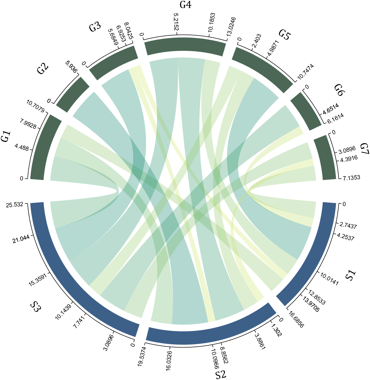
I have written two tools and uploaded fileexchange, which allows us to easily draw chord diagrams:

chord chart 弦图
download:
demo:
dataMat=[2 0 1 2 5 1 2;
3 5 1 4 2 0 1;
4 0 5 5 2 4 3];
dataMat=dataMat+rand(3,7);
dataMat(dataMat<1)=0;
colName={'G1','G2','G3','G4','G5','G6','G7'};
rowName={'S1','S2','S3'};
CC=chordChart(dataMat,'rowName',rowName,'colName',colName);
CC=CC.draw();
CC.setFont('FontSize',17,'FontName','Cambria')
% 显示刻度和数值
% Displays scales and numeric values
CC.tickState('on')
CC.tickLabelState('on')
% 调节标签半径
% Adjustable Label radius
CC.setLabelRadius(1.4);
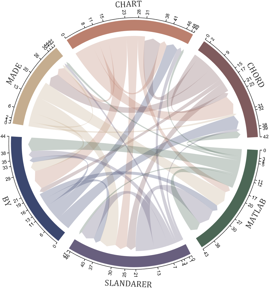
Digraph chord chart 有向弦图
download:
demo:
dataMat=randi([0,8],[6,6]);
% 添加标签名称
NameList={'CHORD','CHART','MADE','BY','SLANDARER','MATLAB'};
BCC=biChordChart(dataMat,'Label',NameList,'Arrow','on');
BCC=BCC.draw();
% 添加刻度
BCC.tickState('on')
% 修改字体,字号及颜色
BCC.setFont('FontName','Cambria','FontSize',17,'Color',[.2,.2,.2])
BCC.setLabelRadius(1.3);
BCC.tickLabelState('on')
There will be a warning when we try to solve equations with piecewise:
syms x y
a = x+y;
b = 1.*(x > 0) + 2.*(x <= 0);
eqns = [a + b*x == 1, a - b == 2];
S = solve(eqns, [x y]);
% 错误使用 mupadengine/feval_internal
% System contains an equation of an unknown type.
%
% 出错 sym/solve (第 293 行)
% sol = eng.feval_internal('solve', eqns, vars, solveOptions);
%
% 出错 demo3 (第 5 行)
% S=solve(eqns,[x y]);
But I found that the solve function can include functions such as heaviside to indicate positive and negative:
syms x y
a = x+y;
b = floor(heaviside(x)) - 2*abs(2*heaviside(x) - 1) + 2*floor(-heaviside(x)) + 4;
eqns = [a + b*x == 1, a - b == 2];
S = solve(eqns, [x y])
% S =
% 包含以下字段的 struct:
%
% x: -3/2
% y: 11/2
The piecewise function is divided into two sections, which is so complex, so this work must be encapsulated as a function to complete:
function pwFunc=piecewiseSym(x,waypoint,func,pfunc)
% @author : slandarer
gSign=[1,heaviside(x-waypoint)*2-1];
lSign=[heaviside(waypoint-x)*2-1,1];
inSign=floor((gSign+lSign)/2);
onSign=1-abs(gSign(2:end));
inFunc=inSign.*func;
onFunc=onSign.*pfunc;
pwFunc=simplify(sum(inFunc)+sum(onFunc));
end
Function Introduction
- x : Argument
- waypoint : Segmentation point of piecewise function
- func : Functions on each segment
- pfunc : The value at the segmentation point
example
syms x
% x waypoint func pfunc
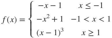
f=piecewiseSym(x,[-1,1],[-x-1,-x^2+1,(x-1)^3],[-x-1,(x-1)^3]);
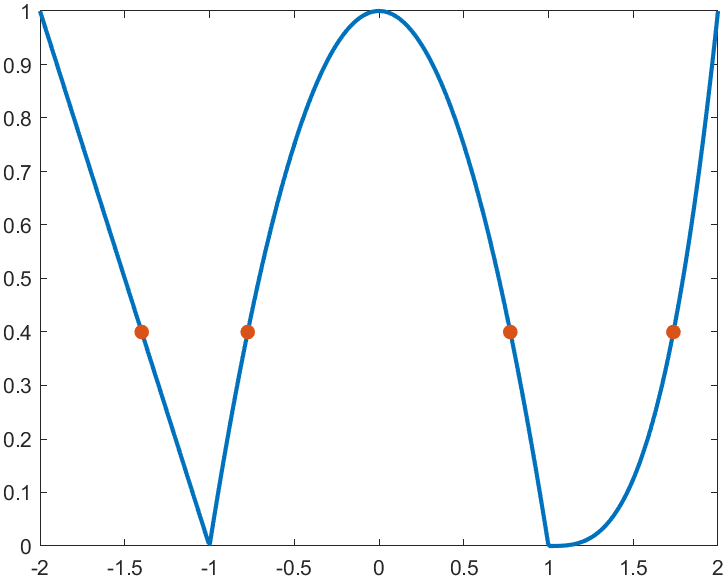
For example, find the analytical solution of the intersection point between the piecewise function and f=0.4 and plot it:
syms x
% x waypoint func pfunc
f=piecewiseSym(x,[-1,1],[-x-1,-x^2+1,(x-1)^3],[-x-1,(x-1)^3]);
% solve
S=solve(f==.4,x)
% S =
%
% -7/5
% (2^(1/3)*5^(2/3))/5 + 1
% -15^(1/2)/5
% 15^(1/2)/5
% draw
xx=linspace(-2,2,500);
f=matlabFunction(f);
yy=f(xx);
plot(xx,yy,'LineWidth',2);
hold on
scatter(double(S),.4.*ones(length(S),1),50,'filled')
precedent
syms x y
a=x+y;
b=piecewiseSym(x,0,[2,1],2);
eqns = [a + b*x == 1, a - b == 2];
S=solve(eqns,[x y])
% S =
% 包含以下字段的 struct:
%
% x: -3/2
% y: 11/2
About Tips & Tricks
Looking to improve your skills and efficiency? Reach your coding goals quickly and more easily with how-tos, tutorials, and shortcuts posted by our staff and community power users.Do you have your own tips and tricks to share? Help other community users with your insights and experience.