Why use Bode plots for designing control systems?
From the series: Understanding Bode Plots
Learn how frequency domain analysis helps you understand the behavior of physical systems in this MATLAB® Tech Talk by Carlos Osorio. You will learn about Bode plots and how they are used by control engineers to gain insights into the behavior of dynamic systems. The Bode plot is a popular tool with control system engineers because it lets them achieve desired closed-loop system performance by graphically shaping the open-loop frequency response using clear and easy-to-understand rules.
Published: 26 Mar 2013
Hi. In this series of videos, I’m going to try to connect some of the basic theory behind the fundamentals of frequency domain analysis with its applications in practice, and the use of tools like Bode plots in the design of typical controllers. I thought that the best way to explain some of the reasons why control or signal processing engineers need to look at things in the frequency domain to begin with would be by using a couple of simple examples.
Let me start with an acoustic guitar, and please, forgive my overly simplistic drawing back there. If we place a microphone anywhere close to its soundboard and we pluck one of the strings, the vibration will resonate in the guitar cavity and will produce a sound wave that will be captured by the mic. Looking at the time trace of that signal from the microphone gives us very little information about what is going on. Only when we look at that same signal on a spectrum analyzer, or we take an FFT of it, we are able to see an amplitude peak and some frequency. This frequency happens to be the underlying tone that forms the note we just played. When you adjust the tuner knob or press your finger at the neck of the guitar, what you’re actually doing is either changing the preload or the effective length of that string. This will shift up or down the frequency at which the string resonates, and you will end up producing a different note.
If we look at a more typical controls example, what I have drawn here is what is known as a two-degrees-of-freedom quarter car suspension. The top mass represents a corner of the car chassis, and the bottom mass represents the corresponding tire. We can use Newton’s Law to come up with a set of differential equations that describe the dynamics of this system. And we can quickly build a model of these equations in a dynamic simulation environment like Simulink. When I press play, the differential equations in the model are stepped through a numerical solver, and we can monitor any of the states of our system. For this simulation run, we are injecting random noise road profile under the tire—think of the car driving over some rough terrain—and we are measuring the acceleration transmitted onto the car body. So, from our numeric simulation solution, we got random noise in and something that looks like a slightly different random noise out. Useful, maybe, but definitely incomplete. I mean, of course, with that dynamic model, we can run more simulations with different types of road profiles and compare the results, but still. I know all the information is there, but it is somewhat hidden underneath those time traces.
Here’s where the genius of people like Fourier and Laplace comes into play: A Laplace transform, for example, will help us convert this forced differential equation problem that can be very difficult to work with in the time domain into a simpler algebraic set of expressions based on the complex Laplace operator, s. Once in the frequency domain, we can easily create a plot of the response of the system for a bunch of different frequencies. You can think of this diagram as the ratio of the amplitude of the energy transmitter from the road under the tire up to the acceleration of the car body.
Actually, what we’re looking at here is pretty typical behavior of any standard car suspension. The first peak corresponds to the resonant frequency of the suspension itself, and the second corresponds to the resonant frequency of the tire. For anybody that has ever wandered off the freeway on to one of those rumble strips on the emergency lane and felt that the car beginning to shake so bad that it felt like it was going to fall apart: The reason why that happened was that the speed of the car, combined with the road profile underneath, was generating an excitation that was probably very close to the resonant frequency of the tire.
By the way, the bumps under the car don’t need to be really big. The critical factor here is the frequency of the excitations. If you hit that rumble strip at the right speed, those tiny bumps can produce very large vertical acceleration jolts on the chassis. And even though those strips are designed to make you instinctively slow down, sometimes, as you take your foot off the gas, you can feel the shaking become even worse before it starts to get better. That is probably because, as the car slows down, the frequency of the excitation also goes down. And if you were on the right-hand side of that second peak to begin with, you will be climbing back up that tire resonance. I know it might sound counterintuitive but notice that if you were to speed up instead, you would be moving further right and down that chart, and the system would completely attenuate whatever disturbance is coming from the road.
Anyway, the point I’m trying to make with all of this is that control engineers need to go through the trouble of analyzing things in the frequency domain because it adds a very important dimension to the observations of our system responses. I like to think that looking at systems exclusively in the time domain—which can feel more natural to us—is analogous to a mechanical designer trying to infer the shape of a three-dimensional part by looking at just a single, two-dimensional drawing of one of its sides.